Constraints and Assertions

Consistency Checking of Inputs, Outputs and Intermediates

While the idea of regression testing comes straight from test-driven development, the next idea we want to discuss is associated more with general defensive progamming than TDD. The idea is consistency checking, i.e. verifying that what might otherwise be implicit assumptions are in fact met by adding checks at various points in the process.¹

Initially, we will assume that we are working with tabular data, but the ideas can be extended to other kinds of data.

Inputs. It is useful to perform some basic checks on inputs. Typical things to consider include:

1. Are the names and types fields in the input data as we expect? In most cases, we also expect field names to be distinct, and perhaps to conform to some rules.

2. Is the distribution of values in the fields reasonable? For example, are the minimum and maximum values reasonable?

3. Are there nulls (missing values) in the data, and if so, are they permitted where they occur? If so, are there any restrictions (e.g. may all the value for a field or record be null?)

4. Is the volume of data reasonable (exactly as expected, if there is a specific size expectation, or plausible, if the volume is variable)?

5. Is any required metadata² included?

In addition to basic sense checks like these, we can also often formulate self-consistency checks on the data. For example:

1. Are any of the fields identifiers or keys for which every value should occur only once?³

2. Are there row-level identities that should be true? For example, we might have a set of category counts and an overall total, and expect the category totals to sum to the overall total:

   nCategoryA + nCategoryB + nCategoryC = nOverall
   

3. For categorical data, are all the values found in the data allowed, and are any required values missing?

4. If the data has a time structure, are the times and dates self-consistent? For example, do any end dates precede start dates? Are there impossible future dates?

5. Are there any ordering constraints on the data, and if so are they respected?

Our goal in formulating TDDA is pragmatic: we are not suggesting it is necessary to check for every possible inconsistency in the input data. Rather, we propose that even one or two simple, well-chosen checks can catch a surprising number of problems. As with regression testing, an excellent time to add new checks is when you discover problems. If you add a consistency check every time you discover bad inputs that such a test would have caught, you might quickly build up a powerful, well-targeted set of diagnostics and verification procedures. As we will see below, there is also a definite possibility of tool support in this area.

Intermediate Results and Outputs. Checking intermediates and outputs is very similar to checking inputs, and all same kinds of tests can be applied. Some further questions to consider in these contexts include:

1. If we look up reference data, do (and should) all the lookups succeed? And are failed lookups handled appropriately?

2. If we calculate a set of results that should exhibit some identity properties, do those hold? Just as physics has conservation laws for quantities such as energy and momentum, there are similar conservation principles in some analytical calculations. As a simple example, if we categorize spending into different, non-overlapping categories, the sum of the category totals should usually equal the sum of all the transactions, as long as we are careful about things like non-categorized values.

3. If we build predictive models, do they cross-validate correctly (if we split the data into a training subset and a validation subset)? And, ideally, do they also validate longitudinally (i.e., on later data, if this is available)?

Transfer checks. With data analysis, our inputs are frequently generated by some other system or systems. Often those systems already perform some checking or reporting of the data they produce. If any information about checks or statistics from source systems is available, it is useful to verify that equivalent statistics calculated over the input data produce the same results. If our input data is transactional, maybe the source system reports (or can report) the number or value of transactions over some time period. Perhaps it breaks things down by category. Maybe we know other summary statistics or there are checksums available that can be verified.

The value of checking that the data received is the same as the data the source system was supposed to send is self-evident, and can help us to detect a variety of problems including data loss, data duplication, data corruption, encoding issues, truncation errors and conversion errors, to name but a few.

Tool Support: Automatic constraint suggestion

A perennial obstacle to better testing is the perception that it is a "nice to have", rather than a sine qua non, and that implementing it will require much tedious work. Because of this, any automated support that tools could provide would seem to be especially valuable.

Fortunately, there is low-hanging fruit in many areas, and one of of our goals with this blog is to explore various tool enhancements. We will do this first in our own Miró software and then, as we find things that work, will try to produce some examples, libraries and tools for broader use, probably focused around the Python data analysis stack.

In the spirit of starting simply, we're first going to look at what might be possible by way of automatic input checking.

One characteristic of data analysis is that we often start by trying to get a result from some particular dataset, rather than setting out to implement an analytical process to be used repeatedly with different inputs. In fact, when we start, we may not even have a very specific analytical goal in mind: we may simply have some data (perhaps poorly documented) and perform exploratory analysis with some broad analytical goal in mind. Perhaps we will stop when we have a result that seems useful, and which we have convinced ourselves is plausible. At some later point, we may get a similar dataset (possibly pertaining to a later period, or a different entity) and need to perform a similar analysis. It's at this point we may go back to see whether we can re-use our previous, embryonic analytical process, in whatever form it was recorded.

Let's assume, for simplicity, that the process at least exists as some kind of executable script, but that it's "hard-wired" to the previous data. We then have three main choices.

• Edit the script (in place) to make it work with the new input data.

• Take a copy of the script and make that work with the new input data.

• Modify the script to allow it to work with either the new or the old data, by parameterizing and generalizing it.

Presented like this, the last sounds like the only sensible approach, and in general it is the better way forward. However, we've all taken the other paths from time to time, often because under pressure just changing a few old hard-wired values to new hard-wired values seems as if it will get us to our immediate result faster.⁴

The problem is that even if were very diligent when preparing the first script, in the context of the original analysis, it is easy for there to be subtle differences in a later dataset that might compromise or invalidate the analysis, and it's hard to force ourselves to be as vigilent the second (third, fourth, ...) time around.

A simple thing that can help is to generate statements about the original dataset and record these as constraints. If a later dataset violates these constraints, it doesn't necessarily mean that anything is wrong, but being alerted to the difference at least offers us an opportunity to consider whether this difference might be significant or problematical, and indeed, whether it might indicate a problem with the data.

Concretely: let's think about what we probably know about a dataset whenever we work with it. We'll use the Periodic Table as an example dataset, based on a snapshot of data I extracted from Wikipedia a few years ago. This is how Miró summarizes the dataset if we ask for a "long" listing of the fields with its ls -l command:

             Field      Type                        Min                         Max    Nulls
                 Z       int                          1                          92       0
              Name    string                   Actinium                   Zirconium       0
            Symbol    string                         Ac                          Zr       0
            Period       int                          1                           7       0
             Group       int                          1                          18      18
    ChemicalSeries    string                   Actinoid            Transition metal       0
      AtomicWeight      real                       1.01                      238.03       0
         Etymology    string                      Ceres                      zircon       0
RelativeAtomicMass      real                       1.01                      238.03       0
     MeltingPointC      real                    -258.98                    3,675.00       1
MeltingPointKelvin      real                      14.20                    3,948.00       1
     BoilingPointC      real                    -268.93                    5,596.00       0
     BoilingPointF      real                    -452.07                   10,105.00       0
           Density      real                       0.00                       22.61       0
       Description    string                        0.2            transition metal      40
            Colour    string    a soft silver-white ...    yellowish green or g ...      59

For each field, we have a name, a type, minimum and maximum values and a count of the number of missing values. [Scroll sideways if your window is too narrow to see the Nulls column on the right.] We also have, implicitly, the field order.

This immediately suggests a set of constraints we might want to construct. We've added an experimental command to Miró for generating constraints based on the field metadata shown earlier and a few other statistics. First, here's the "human-friendly" view that Miró produces if we use its autoconstraints -l command.

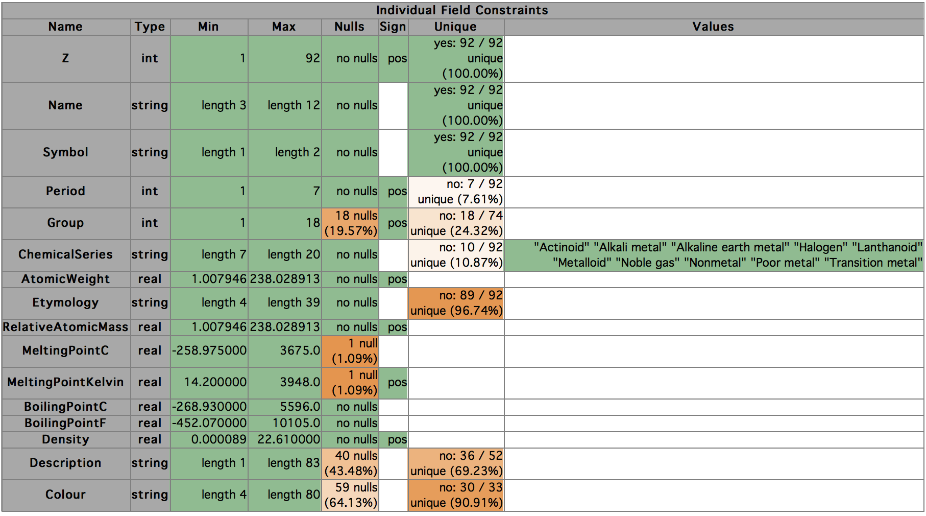
In this table, the green cells represent constraints the system suggests for fields, and the orange cells show areas in which potential constraints were not constructed, though they would have been had the data been different. Darker shades of orange indicate constraints that were closer to be met within the data.

In addition to this human-friendly view, Miró generates out a set of declarations, which can be thought of as candidate assertions. Specifically, they are statements that are true in the current dataset, and therefore constitute potential checks we might want to carry out on any future input datasets we are using for the same analytical process.

Here they are:

declare (>= (min Z) 1)
declare (<= (max Z) 92)
declare (= (countnull Z) 0)
declare (non-nulls-unique Z)

declare (>= (min (length Name)) 3)
declare (<= (min (length Name)) 12)
declare (= (countnull Name) 0)
declare (non-nulls-unique Name)

declare (>= (min (length Symbol)) 1)
declare (<= (min (length Symbol)) 2)
declare (= (countnull Symbol) 0)
declare (non-nulls-unique Symbol)

declare (>= (min Period) 1)
declare (<= (max Period) 7)
declare (= (countnull Period) 0)

declare (>= (min Group) 1)
declare (<= (max Group) 18)

declare (>= (min (length ChemicalSeries)) 7)
declare (<= (min (length ChemicalSeries)) 20)
declare (= (countnull ChemicalSeries) 0)
declare (= (countzero
            (or (isnull ChemicalSeries)
                (in ChemicalSeries (list "Actinoid" "Alkali metal"
                                         "Alkaline earth metal"
                                         "Halogen" "Lanthanoid"
                                         "Metalloid" "Noble gas"
                                         "Nonmetal" "Poor metal"
                                         "Transition metal"))))
           0)

declare (>= (min AtomicWeight) 1.007946)
declare (<= (max AtomicWeight) 238.028914)
declare (= (countnull AtomicWeight) 0)
declare (> (min AtomicWeight) 0)

declare (>= (min (length Etymology)) 4)
declare (<= (min (length Etymology)) 39)
declare (= (countnull Etymology) 0)

declare (>= (min RelativeAtomicMass) 1.007946)
declare (<= (max RelativeAtomicMass) 238.028914)
declare (= (countnull RelativeAtomicMass) 0)
declare (> (min RelativeAtomicMass) 0)

declare (>= (min MeltingPointC) -258.975000)
declare (<= (max MeltingPointC) 3675.0)

declare (>= (min MeltingPointKelvin) 14.200000)
declare (<= (max MeltingPointKelvin) 3948.0)
declare (> (min MeltingPointKelvin) 0)

declare (>= (min BoilingPointC) -268.930000)
declare (<= (max BoilingPointC) 5596.0)
declare (= (countnull BoilingPointC) 0)

declare (>= (min BoilingPointF) -452.070000)
declare (<= (max BoilingPointF) 10105.0)
declare (= (countnull BoilingPointF) 0)

declare (>= (min Density) 0.000089)
declare (<= (max Density) 22.610001)
declare (= (countnull Density) 0)
declare (> (min Density) 0)

declare (>= (min (length Description)) 1)
declare (<= (min (length Description)) 83)

declare (>= (min (length Colour)) 4)
declare (<= (min (length Colour)) 80)

Each green entry in the table maps to a declaration in this list. Let's look at a few:

1. Min and Max. Z is the atomic number. Each element has an atomic number, which is the number of protons in the nucleus, and each is unique. Hydrogen has the smallest number of protons, 1, and in this dataset, Uranium has the largest number—92. So the first suggested constraints are that these values should be in the observed range. These show up as the first two declarations:

   declare (>= (min Z) 1)
   declare (<= (max Z) 92)
   

   We should say a word about how these constraints are expressed. Miró includes expression language called (lisp-like), (because it's essentially a dialect of Lisp). Lisp is slightly unusual in that instead of writing f(x, y) you write (f x y). So the first expression would be more commonly expressed as

   min(Z) >= 1
   

   in regular ("infix") languages.

   Lisp weirdness aside, are these sensible constraints? Well, the first certainly is. Even if we find some elements beyond Uranium (which we will, below), we certainly don't expect them to have zero or negative numbers of protons, so the first constraint seems like a keeper.

   The second constraint is much less sensible. In fact, given that we know the dataset includes every value of Z from 1 to 92, we confidently expect that any future revisions of the periodic table will include values higher than 92. So we would probably discard that constraint.

   The crucial point is that no one wants to sit down and write out a bunch of constraints by hand (and anyway, "why have a dog an bark yourself?"). People are generally much more willing to review a list of suggested constraints and delete the ones that don't make sense, or modify them so that they do.

2. Nulls. The next observation about Z is that it contains no nulls. This turns into the (lisp-like) constraint:

   declare (= (countnull Z) 0)
   

   This is also almost certainly a keeper: we'd probably be pretty unhappy if we received a Periodic Table with missing Z values for any elements.

   (Here, (countnull Z) just counts the number of nulls in field Z, and = tests for equality, so the expression reads "the number of nulls in Z is equal to zero".)

3. Sign. The sign column is more interesting. Here, we have recorded the fact that all the values in Z are positive. Clearly, this is a logically implied by the fact that the minimum value for Z is 1, but we think it's useful to record two separate observations about the field—first, that its minimum value is 1, and secondly that it is always strictly positive. In cases where the minimum is 1, for an integer field, these statements are entirely equivalent, but if the minimum had been (say) 3, they would be different. The value of recording these observations separately arises if at some later stage the minimum changes, while remaining positive. In that case, we might want to discard the specific minimum constraint, but leave in place the constraint on the sign.

   Although we record the sign as a separate constraint in the table, in this case it does not generate a separate declaration, as it would be identical to the constraint on the minimum that we already have.

   In contrast, AtomicWeight, has a minimum value around 1.008, so it does get a separate sign constraint:

   declare (> (min AtomicWeight) 0)
   

4. Uniqueness of Values. The next thing our autoconstraints framework has noticed about Z is that none of its values is repeated in the data—that all are unique (a.k.a. distinct). The table reports this as yes (the values are unique) and 92/92 (100%), meaning that there are 92 distinct values and 92 non-null values in total, so that 100% of values are unique. Other fields, such as Etymology, have potential constraints that are not quite met: Etymology has 89 different values in the field, so the ratio of distinct values to values is about 97%.

   NOTE: in considering this, we ignore nulls if there are any. You can see this if you look at the Unique entry for the field Group: here there are 18 different (non-null) values for Group, and 74 records have non-null values for Group.

   There is a dedicated function in (lisp-like) for checking whether the non-null values in a field are all distinct, so the expression in the declaration is just:

   (non-nulls-unique Z)
   

   which evaluates to true⁵ or false.

5. Min and Max for String Fields. For string fields, the actual minimum and maximum values are usually less interesting. (Indeed, there are lots of reasonable alternative sort orders for strings, given choices such as case sensitivity, whether embedded numbers should be sorted numerically or alphanumerically, how spaces and punctuation should be handled, what to do with accents etc.) In the initial implementation, instead of using any min and max string values as the basis of constraints, we suggest constraints based on string length.

   For the string fields here, none of the constraints is particularly compelling, though a minimum length of 1 might be interesting and you might even think that a maximum length of 2 is sensible the symbol is useful. But in many cases they will be. One common case is fixed-length strings, such as the increasingly ubiquitous UUIDs,⁶ where the minimum and maximum values would both 36 if they are canonically formatted. (Of course, we can add much stronger constraints if we know all the strings in a field are UUIDs.)

6. Categorical Values. The last kind of automatically generated constraint we will discuss today is a restriction of the values in a field to be chosen from some fixed set. In this case, Miró has noticed that there are only 10 different non-null values for ChemicalSeries, so has suggested a constraint to capture that reality. The slightly verbose way this currently gets expressed as a constraint is:

   declare (= (countzero
               (or (isnull ChemicalSeries)
                   (in ChemicalSeries
                       (list "Actinoid" "Alkali metal"
                             "Alkaline earth metal"
                             "Halogen" "Lanthanoid" "Metalloid" "Noble gas"
                             "Nonmetal" "Poor metal" "Transition metal"))))
              0)
   

   (The or statement starting on the second line is true for field values that are either in the list or null. The countzero function, when applied to booleans, counts false values, so this is saying that none of the results of the or statement should be false, i.e. all values should be null or in the list. This would be more elegantly expressed with an (all ...) statement; we will probably change it to that formulation soon, though the current version is more useful for reporting failures.)

   The current implementation generates these constraints only when the number of distinct values it sees is 20 or fewer, only for string fields, and only when not all the values in the field are distinct, but all of these aspect can probably be improved, and the user can override the number of categories to allow.

In addition to these constraints, we should also probably generate constraints on the field types and, as we will discuss in future articles, dataset-level constraints.

Tool Support: Using the Declarations

Obviously, if we run test the constraints against the same dataset we used to generate them, all the constraints should be (and are!) satisfied. Things are slightly more interesting if we run them against a different dataset. In this case, we excluded transuranic elements from the dataset we used to generate the constraints. But we can add them in. If we do so, and then execute a script (e92.miros) containing the autogenerated constraints, we get the following output:

$ miro
This is Miro, version 2.1.90.
Copyright © Stochastic Solutions 2008-2015.
Seed: 1463187505
Logs started at 2015/11/25 17:08:23 host tdda.local.
Logging to /Users/njr/miro/log/2015/11/25/session259.

[1]> load elements
elements.miro: 118 records; 118 (100%) selected; 16 fields.
[2]> . e92
[3]> # Autoconstraints for dataset elements92.miro.
[4]> # Generated from session /Users/njr/miro/log/2015/11/25/session256.miros
[5]> declare (>= (min Z) 1)
[6]> declare (<= (max Z) 92)

Miro Warning: Declaration failed: (<= (max Z) 92)

[7]> declare (= (countnull Z) 0)
[8]> declare (non-nulls-unique Z)
[9]> declare (>= (min (length Name)) 3)
[10]> declare (<= (min (length Name)) 12)
[11]> declare (= (countnull Name) 0)
[12]> declare (non-nulls-unique Name)
[13]> declare (>= (min (length Symbol)) 1)
[14]> declare (<= (min (length Symbol)) 2)
[15]> declare (= (countnull Symbol) 0)
[16]> declare (non-nulls-unique Symbol)
[17]> declare (>= (min Period) 1)
[18]> declare (<= (max Period) 7)
[19]> declare (= (countnull Period) 0)
[20]> declare (>= (min Group) 1)
[21]> declare (<= (max Group) 18)
[22]> declare (>= (min (length ChemicalSeries)) 7)
[23]> declare (<= (min (length ChemicalSeries)) 20)
[24]> declare (= (countnull ChemicalSeries) 0)
[25]> declare (= (countzero
                  (or (isnull ChemicalSeries)
                      (in ChemicalSeries (list "Actinoid" "Alkali metal"
                                               "Alkaline earth metal"
                                               "Halogen" "Lanthanoid"
                                               "Metalloid" "Noble gas"
                                               "Nonmetal" "Poor metal"
                                               "Transition metal"))))
                 0)
[26]> declare (>= (min AtomicWeight) 1.007946)
[27]> declare (<= (max AtomicWeight) 238.028914)

Miro Warning: Declaration failed: (<= (max AtomicWeight) 238.028914)

[28]> declare (= (countnull AtomicWeight) 0)

Miro Warning: Declaration failed: (= (countnull AtomicWeight) 0)

[29]> declare (> (min AtomicWeight) 0)
[30]> declare (>= (min (length Etymology)) 4)
[31]> declare (<= (min (length Etymology)) 39)
[32]> declare (= (countnull Etymology) 0)

Miro Warning: Declaration failed: (= (countnull Etymology) 0)

[33]> declare (>= (min RelativeAtomicMass) 1.007946)
[34]> declare (<= (max RelativeAtomicMass) 238.028914)

Miro Warning: Declaration failed: (<= (max RelativeAtomicMass) 238.028914)

[35]> declare (= (countnull RelativeAtomicMass) 0)

Miro Warning: Declaration failed: (= (countnull RelativeAtomicMass) 0)

[36]> declare (> (min RelativeAtomicMass) 0)
[37]> declare (>= (min MeltingPointC) -258.975000)
[38]> declare (<= (max MeltingPointC) 3675.0)
[39]> declare (>= (min MeltingPointKelvin) 14.200000)
[40]> declare (<= (max MeltingPointKelvin) 3948.0)
[41]> declare (> (min MeltingPointKelvin) 0)
[42]> declare (>= (min BoilingPointC) -268.930000)
[43]> declare (<= (max BoilingPointC) 5596.0)
[44]> declare (= (countnull BoilingPointC) 0)

Miro Warning: Declaration failed: (= (countnull BoilingPointC) 0)

[45]> declare (>= (min BoilingPointF) -452.070000)
[46]> declare (<= (max BoilingPointF) 10105.0)
[47]> declare (= (countnull BoilingPointF) 0)

Miro Warning: Declaration failed: (= (countnull BoilingPointF) 0)

[48]> declare (>= (min Density) 0.000089)
[49]> declare (<= (max Density) 22.610001)

Miro Warning: Declaration failed: (<= (max Density) 22.610001)

[50]> declare (= (countnull Density) 0)

Miro Warning: Declaration failed: (= (countnull Density) 0)

[51]> declare (> (min Density) 0)
[52]> declare (>= (min (length Description)) 1)
[53]> declare (<= (min (length Description)) 83)
[54]> declare (>= (min (length Colour)) 4)
[55]> declare (<= (min (length Colour)) 80)

10 warnings and 0 errors generated.

Job completed after a total of 10.2801 seconds.
Logs closed at 2015/11/25 17:08:23 host tdda.local.
Logs written to /Users/njr/miro/log/2015/11/25/session259.

By default, Miró generates warnings when declared constraints are violated. In this case, ten of the declared constraints were not met, so there were ten warnings. We can also set the declarations to generate errors rather than warnings, allowing us to stop execution of a script if the data fails to meet our declared expectations.

In this case, the failed declarations are mostly unsurprising and untroubling. The maximum values for Z, AtomicWeight, RelativeAtomicMass, and Density all increase in this version of the data, which is expected given that all the new elements are heavier than those in the initial analysis set. Equally, while the fields AtomicWeight, RelativeAtomicMass, Etymology, BoilingPointC, BoilingPointF and Density were all populated in the original dataset, each now contains nulls. Again, this is unsurprising in this case, but in other contexts, detecting these sorts of changes in a feed of data might be important. Specifically, we should always be interested in unexpected differences between the datasets used to develop an analytical process, and ones for which that process is used at a later time: it is very possible that they will not be handled correctly if they were not seen or considered when the process was developed.

There are many further improvements we could make to the current state of the autoconstraint generation, and there are other kinds of constraints it can generate that we will discuss in later posts. But as simple as it is, this level of checking has already identified a number of problems in the work we have been carrying out with Skyscanner and other clients.

We will return to this topic, including discussing how we might add tool support for revising constraint sets in the light of failures, merging different sets of constraints and adding constraints that are true only of subsets of the data.

Parting thoughts

Outputs and Intermediates. While developing the ideas about automatically generating constraints, our focus was mostly on input datasets. But in fact, most of the ideas are almost as applicable to intermediate results and outputs (which, after all, often form the inputs to the next stage of an analysis pipeline). We haven't performed any analysis in this post, but if we had, there might be similar value in generating constraints for the outputs as well.

Living Constraints and Type Systems. In this article, we've also focused on checking constraints at particular points in the process—after loading data, or after generating results. But it's not too much of a stretch to think of constraints as statements that should always be true of data, even as we append records, redefine fields etc. We might call these living or perpetual constraints. If we do this, individual field constraints become more like types. This idea, together with dimensional analysis, will be discussed in future posts.