Almost all data scientists and data engineers have to work with flat files (CSV files) from time to time. Despite their many problems, CSVs are too ubiquitous, too universal, and (whisper it) have too many strengths for them to be likely to disappear. Even if they did, they would quickly be reinvented. The problems with them are widely known and discussed, and will be familar to almost everyone who works with them. They include issues with encodings, types, quoting, nulls, headers, and with dates and times. My favourite summary of them remains Jesse Donat's Falsehoods Programmers Believe about CSVs. I wrote about them on this blog nearly four years ago (Flat Files).

Over the last year or so I've been writing a book on test-driven data analysis. The only remaining chapter without a full draft discusses the same topics as this post—metadata for CSV files and new parts of the TDDA software that assist with its creation and use. This post documents my current thinking, plans and ambitions in this area, and shows some of what is already implemented.¹

A Metadata Format for Flat Files: tdda.serial

The core of the new work is a new format, tdda.serial, for describing data in CSV files.

The previous post showed an example (“XMD”) metadata file used by the Miró software from my company Stochastic Solutions, which was as follows:²

    <?xml version="1.0" encoding="UTF-8"?>
    <dataformat>
        <sep>,</sep>                     <!-- field separator -->
        <null></null>                    <!-- NULL marker -->
        <quoteChar>"</quoteChar>         <!-- Quotation mark -->
        <encoding>UTF-8</encoding>       <!-- any python coding name -->
        <allowApos>True</allowApos>      <!-- allow apostophes in strings -->
        <skipHeader>False</skipHeader>   <!-- ignore the first line of file -->
        <pc>False</pc>                   <!-- Convert 1.2% to 0.012 etc. -->
        <excel>False</excel>             <!-- pad short lines with NULLs -->
        <dateFormat>eurodt</dateFormat>  <!-- Miró date format name -->
        <fields>
            <field extname="mc id" name="ID" type="string"/>
            <field extname="mc nm" name="MachineName" type="int"/>
            <field extname="secs" name="TimeToManufacture" type="real"/>
            <field extname="commission date" name="DateOfCommission"
                   type="date"/>
            <field extname="mc cp" name="Completion Time" type="date"
                   format="rdt"/>
            <field extname="sh dt" name="ShipDate" type="date" format="rd"/>
            <field extname="qa passed?" name="Passed QA" type="bool"/>
        </fields>
        <requireAllFields>False</requireAllFields>
        <banExtraFields>False</banExtraFields>
    </dataformat>

Here is one equivalent way of expressing essentially the same information in the (evolving) tdda.serial format:

{
    "format": "http://tdda.info/ns/tdda.serial",
    "writer": "tdda.serial-2.2.15",
    "tdda.serial": {
        "encoding": "UTF-8",
        "delimiter": "|",
        "quote_char": "\"",
        "escape_char": "\\",
        "stutter_quotes": false,
        "null_indicators": "",
        "accept_percentages_as_floats": false,
        "header_row_count": 1,
        "map_missing_trailing_cols_to_null": false,
        "fields": {
            "mc id": {
                "name": "ID",
                "fieldtype": "int"
            },
            "mc nm": {
                "name": "Name",
                "fieldtype": "string"
            },
            "secs": {
                "name": "TimeToManufacture",
                "fieldtype": "int"
            },
            "commission date": {
                "name": "DateOfCommission",
                "fieldtype": "date",
                "format": "iso8601date"
            },
            "mc cp": {
                "name": "CompletionTime",
                "fieldtype": "datetime",
                "format": "iso8601datetime"
            },
            "sh dt":  {
                "name": "ShipDate",
                "fieldtype": "date",
                "format": "iso8601date"
            },
            "qa passed?": {
                "name": "PassedQA",
                "fieldtype": "bool",
                "true_values": "yes",
                "false_values": "no"
            }
        }
    }
}

The details don't matter too much at this stage, and may yet change, but briefly here we see the file (typically with a .serial extension), describing:

• the text encoding used for the data (UTF-8);
• the field separator (pipe, |);
• the quote character (double quote, ");
• the escape character (\), which is used to escape double quotes in double-quoted strings, among other things;
• whether quotes are stuttered or escaped within quoted strings;
• the string used to denote null values (this can be a single string or a list);
• the number of header rows;
• an explicit note not to accept percentages in the file as floating-point values;
• whether or not lines with too few fields should be regarded as having nulls for the apparently missing fields. (Excel usually does not write values after the last non-empty cell in each row on a worksheet.)
• information about individual fields. In this case, a dictionary is used to map names in the flat file to names to be used in the dataset. Numbers can also be used to indicate column position, particularly if there is no header, though they have to be quoted because this is JSON. Field types are also specified, together with any extra information required, e.g. the non-standard true and false values for the boolean field collected? (in the file), which becomes HasBeenCollected once read. Formats for the date and time fields are also specified here.

When the fields are presented as a dictionary, as here, this allows for the possibility that there are other fields in the file, for which metadata is not provided. If a list is used instead, the field list is taken to be complete. In this case, external names can be provided using an csvname attribute, if they are different.

Pretty much everything is optional, and, where appropriate, defaults can be put in the main section and over-ridden on a per-field basis. This is useful if, for example, one or two fields use different null markers from the default, or if multiple date formats are used. (The format key will probably change to dateformat and boolformat to make this overriding work better.)

Here is a simple example of its use with Pandas. Suppose we have the following pipe-separated flat file, with the name machines.psv.

mc id|mc nm|secs|commission date|mc cp|sh dt|qa passed?
1111111|"Machine 1"|86400|2025-06-01|2025-06-07T12:34:56|2025-06-21|yes
2222222|"Machine 2"||2025-06-02|2025-06-08T12:34:57|2025-06-22
3333333|"Machine 3"|86399|2025-06-03|2025-06-09T12:34:55|2025-06-22|no

Then we can use the following Python code to load the data, informed by the metadata in machines.serial (the example shown above).

from tdda.serial import csv_to_pandas

df = csv_to_pandas('machines.psv', 'machines.serial')
print(df, '\n')
df.info()

This produces the following output:

$ python pd-read-machines.py
        ID       Name  TimeToManufacture DateOfCommission      CompletionTime   ShipDate  PassedQA
0  1111111  Machine 1              86400       2025-06-01 2025-06-07 12:34:56 2025-06-21      True
1  2222222  Machine 2               <NA>       2025-06-02 2025-06-08 12:34:57 2025-06-22      <NA>
2  3333333  Machine 3              86399       2025-06-03 2025-06-09 12:34:55 2025-06-22     False

<class 'pandas.core.frame.DataFrame'>
RangeIndex: 3 entries, 0 to 2
Data columns (total 7 columns):
 #   Column             Non-Null Count  Dtype
---  ------             --------------  -----
 0   ID                 3 non-null      Int64
 1   Name               3 non-null      string
 2   TimeToManufacture  2 non-null      Int64
 3   DateOfCommission   3 non-null      datetime64[ns]
 4   CompletionTime     3 non-null      datetime64[ns]
 5   ShipDate           3 non-null      datetime64[ns]
 6   PassedQA           2 non-null      boolean
dtypes: Int64(2), boolean(1), datetime64[ns](3), string(1)
memory usage: 288.0 bytes

There's nothing particularly special here, but Pandas has read the file correctly using the metadata to understand

• the pipe separator;
• the date and time formats;
• the yes/no format of PassedQA;
• the null indicator;
• the intended, more usable internal field names;
• field types, here defaulting to nullable types.

As with the pandas.read_csv, we can choose whether to prefer nullable types, but the default using tdda.serial is to do so. In this case, the date formats and null indicators would be fine anyway, with Pandas defaults, but here we could instead have specified, say, European dates and ? for nulls.

This code:

from tdda.serial load_metadata, serial_to_pandas_read_csv_args
from rich import print as rprint

md = load_metadata('machines.serial')
kwargs = serial_to_pandas_read_csv_args(md)
rprint(kwargs)

shows the parameters actually passed to pandas.read_csv:

{
    'dtype': {'ID': 'Int64', 'Name': 'string', 'TimeToManufacture': 'Int64', 'PassedQA': 'boolean'},
    'date_format': {'DateOfCommission': 'ISO8601', 'CompletionTime': 'ISO8601', 'ShipDate': 'ISO8601'},
    'parse_dates': ['DateOfCommission', 'CompletionTime', 'ShipDate'],
    'sep': '|',
    'encoding': 'UTF-8',
    'escapechar': '\\',
    'quotechar': '"',
    'doublequote': False,
    'na_values': [''],
    'keep_default_na': False,
    'names': ['ID', 'Name', 'TimeToManufacture', 'DateOfCommission', 'CompletionTime', 'ShipDate', 'PassedQA'],
    'header': 0,
    'true_values': ['yes'],
    'false_values': ['no']
}

We can do the very similar things using Polars (and “soon”, other libraries). Here's a way to read the file with Polars:

from tdda.serial import csv_to_polars

df = csv_to_polars('machines.psv', 'machines.serial',
                   map_other_bools_to_string=True)
print(df)

which produces:

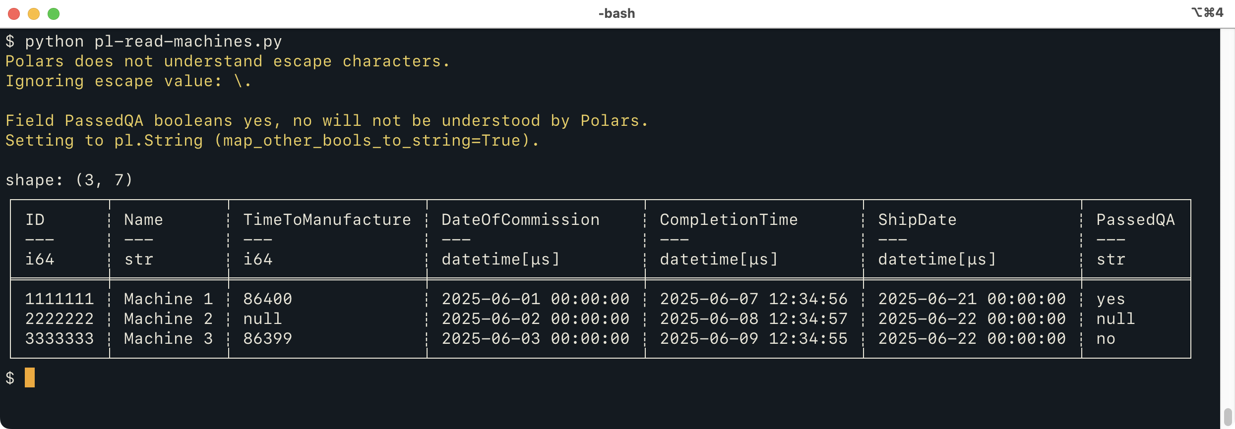
This does mostly the same thing as the Pandas version, but issues two warnings. The first is because an escape character is specified, which the Polars CSV reader doesn't really understand. The second warning is because the Polars CSV reader can't handle non-standard booleans. By default, when these are specified for Polars, tdda.serial will issue a warning but still call polars.read_csv to read the file, because they might not, in fact, be used. The parameter passed in the Python code above (map_other_bools_to_string=True) tells tdda.serial to direct Polars to read this column as a string instead (as it would if we didn't specify a type). Of course, it would be possible to have the reader then go through and turn the strings into booleans after reading, but that feels like more a metadata library should do.

The warnings helpfully tell you what to look out for as possible issues when the file is read. This as an example of a principle I'm trying to use throughout tdda.serial: when there's something in the serial metadata that a given reader might not be able to handle correctly, issue a warning, and possibly provide an option to control that behaviour.

We can do the same thing as we did for Pandas and look at the arguments generated for Polars, using the following, very similar, Python code:

from tdda.serial import (load_metadata, serial_to_polars_read_csv_args)
from rich import print as rprint

md = load_metadata('machines.serial')
kwargs = serial_to_polars_read_csv_args(md, map_other_bools_to_string=True)
rprint(kwargs)

This produces

{
    'separator': '|',
    'quote_char': '"',
    'null_values': [''],
    'encoding': 'UTF-8',
    'schema': {
        'ID': Int64,
        'Name': String,
        'TimeToManufacture': Int64,
        'DateOfCommission': Datetime,
        'CompletionTime': Datetime,
        'ShipDate': Datetime,
        'PassedQA': String
    },
    'new_columns': [
        'ID',
        'Name',
        'TimeToManufacture',
        'DateOfCommission',
        'CompletionTime',
        'ShipDate',
        'PassedQA'
    ]
}

The only subtlety here is that the types in Schema are actual polars types (pl.Int64 etc.) rather than strings, hence their not being quoted. (They're not prefixed because repr(pl.Int64) is the string "Int64", which prints as Int64.) The library can also write a tdda.serial file containing the Polars arguments explicitly. It looks like this:

{
    "format": "http://tdda.info/ns/tdda.serial",
    "writer": "tdda.serial-2.2.15",
    "polars.read_csv": {
        "separator": "|",
        "quote_char": "\"",
        "null_values": [
            ""
        ],
        "encoding": "UTF-8",
        "schema": {
            "ID": "Int64",
            "Name": "String",
            "TimeToManufacture": "Int64",
            "DateOfCommission": "Datetime",
            "CompletionTime": "Datetime",
            "ShipDate": "Datetime",
            "PassedQA": "String"
        },
        "new_columns": [
            "ID",
            "Name",
            "TimeToManufacture",
            "DateOfCommission",
            "CompletionTime",
            "ShipDate",
            "PassedQA"
        ]
    }
}

Here, because we need to serialize the tdda.serial file as JSON, the polars types are mapped to their string names. The tdda library takes care of the conversion in both directions.

A single .serial file can contain multiple flavours of metadata—tdda.serial, polars.read_csv, pandas.read_csv etc. When it does, a call to load_metadata can specify a preferred flavour, or let the library choose. My hope, however, is that in most cases the tdda.serial section will contain enough information to work as well as a library-specific specification.

Goals for tdda.serial

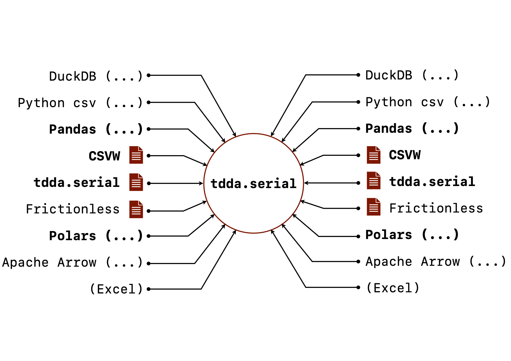
When I went to write down the goals for tdda.serial, I was surprised at how long the list was. Not all of this is implemented but here is the current state of the goals for tdda.serial. (The image above shows the vision for it, with the bold parts mostly implemented, and the rest currently only planned.)

• Describe Flat File Formats. Allow accurate representation, full or partial, of flat-file formats used (or potentially used) by one or more concrete flat files. or .
  • It primarily targets comma-separated values (.csv) and related formats (tab-separated, pipe-separated etc.), but also potentially other tabular data. It could, for example, be used to describe things like date formats and numeric subtypes for tabular data stored in JSON or JSON Lines.
  • Full or partial is important. When reading data, it is often convenient only to specify things that are causing problems. On write, fuller specifications are, of course, desirable.
• Read Flat Files. Assist with reading flat files correctly, based on metadata in .serial files and other formats (like CSVW), primarily using data in the "tdda.serial" format.
  • Convert metadata currently stored as tdda.serial to dictionaries of arguments for other libraries that work with CSVs.
  • Provide an API to get such libraries to read flat-file data correctly, guided by the metadata
  • Generate code to get such libraries to read flat-file data correctly, guided by the metadata. Assist with writing flat files in documented formats.
  • Interoperate, where possible, with other metadata formats like CSVW and Frictionless.
• Generate tdda.serial Metadata Files. Assist with generating metadata describing the format of CSV files based on the write arguments provided to the writing software.
• Write Flat Files. Assist with getting libraries to write CSV files using a format specified in a tdda.serial file.
  • This provides a second way of increasing interoperability: we can help readers to read from a specific format, and writers to write to that same format.
• Assist/Support other Software Reading, Writing, and otherwise handling Flat Files.
  • DataFrame Libraries
    • Pandas
    • Polars
    • Apache Arrow
  • Databases
    • DuckDB
    • SQLite
    • Postgres
    • MySQL
  • Miscellaneous
    • Python csv
    • tdda
• Support Library-specific Read/Write Metadata. Provide a mechanism for documenting library-specific read/write parameters for CSV files explicitly:
  • For storing the library-specific write parameters used with pandas.to_csv, polars.write_csv in .serial files (and the ability to use such parameters)
  • For storing the library-specific read parameters required to read a flat file with high fidelity using, e.g. pandas.read_csv , polars.read_csv etc.
• Assist with Format Choice. Provide a mechanism for helping to choose a good CSV format for a concrete dataset to be written, e.g. choosing null indicators that are not likely to be confused with serialized non-null values in the dataset.
• SERDE Verification. Provide mechanisms for checking whether a dataset can be round-tripped successfully to a flat file (i.e. that the same library, at least, can write data to a flat file, read it back, and recover identical, equivalent, or similar data).³

• CLI Tools. Through the associated command-line tool, tdda diff, and equivalent API functions, to check whether two datasets are equivalent.

  • In the case of the command-line tool this is two datasets on disk (flat files, parquet files etc.). It might also be possible to compare two database tables, in the same or different RDBMS instances, or data in a database table and in a file on disk, though this is not yet implemented. (The next post will discuss tdda diff further.)
  • In the case of the API, this can also include in-memory data structures such as data frames.

• Provide Metadata Format Conversions. Provide mechanisms for converting between different library-specific flat-file parameters and tdda's tdda.serial format, as well as between the tdda.serial format, csvw, and (perhaps) frictionless.

• Generate Validation Statistics and Validate using them. (Potentially) write additional data for a concrete dataset that can be used for further validation that it has been read correctly, e.g. summary statistics, checksums etc.

Discussion

The usual observation when proposing something new like this is that the last thing the world needs is another “standard”. As Randall Munro puts it: (https://imgs.xkcd.com/927):

In this case, however, I don't think there are all that many recognized ways of describing flat-file formats. I was involved in one (the .fdd flat-file description data format) while at Quadstone, and I currently use the XMD format above at Stochastic Solutions, but pretty-much no one else does. While working with a friend, Neil Skilling, he ran across the CSVW standard, developed under the auspices of W3C, and that led to my finding the Python frictionless project. At first I thought one of those might be the solution I was looking for, but in fact they have goals and desgins that are different enough that they don't quite fulfill the most important goals for tdda.serial, as impressive as both projects are. Reluctantly, therefore, I began working on tdda.serial, which aims to interoperate with and support CSVW, (and to some extent, frictionless), but also to handle other cases.

The biggest single difference between the focus of tdda.serial and the CSVW is that tdda.serial is primarily concerned with documenting a format that might be used by many flat files (different concrete datasets sharing the same sttructure and formatting) whereas CSVW is primarily concerned with documenting either a single specific CSV file or a specific collection of CSV files, usually each having different structure. This seems like a rather subtle difference, but in fact turns out to be quite consequential.

Here's the first example CSVW file from csvw.org:

{
  "@context": ["http://www.w3.org/ns/csvw", {"@language": "en"}],
  "tables": [{
    "url": "http://opendata.leeds.gov.uk/downloads/gritting/grit_bins.csv",
    "tableSchema": {
      "columns": [
      {
        "name": "location",
        "datatype": "integer"
      },
      {
        "name": "easting",
        "datatype": "decimal",
        "propertyUrl": "http://data.ordnancesurvey.co.uk/ontology/spatialrelations/easting"
      },
      {
        "name": "northing",
        "datatype": "decimal",
        "propertyUrl": "http://data.ordnancesurvey.co.uk/ontology/spatialrelations/northing"
      }
      ],
      "aboutUrl": "#{location}"
    }
  }],
  "dialect": {
    "header": false
  }
}

Notice that the CSVW file caters for multiple CSV files (a list of tables in the tables element), and that the location of the table is provided as a URL (which is a required element in CSVW). In the context of CSV on the web, this makes complete sense. It's specified as being URL, but can be a file: URL, or a simple path. One convention, fora CSVW file documenting a single dataset, seems to be that the metadata for grit_bins.csv is stored in grit_bins-metadata.json in the same directory as the CSV file itself (locally, or on the web).

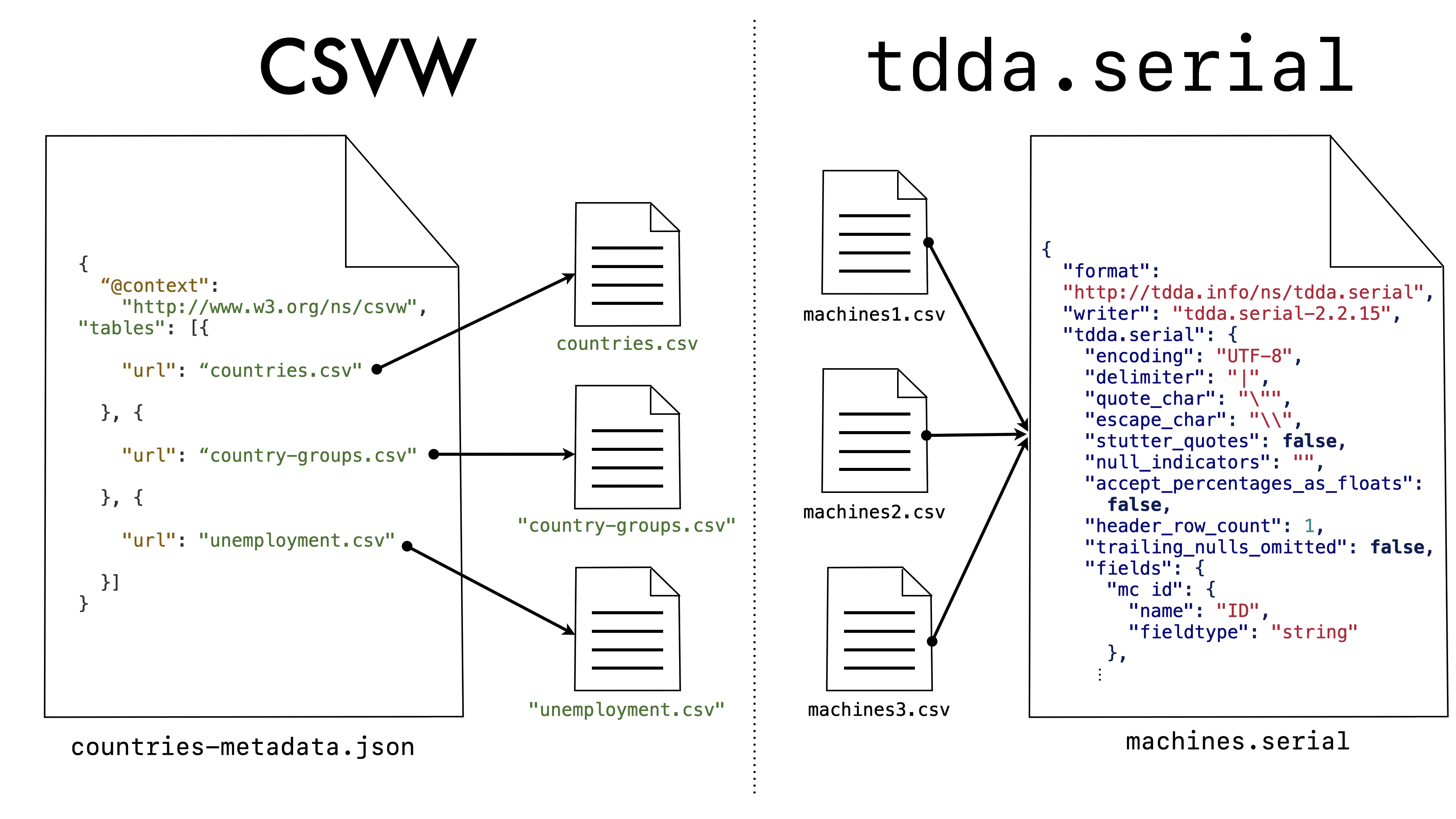
What is significant, however, is that this establishes either a one-to-one relationship between CSV files and CSVW metadata files or, if the CSVW file contains metadata about several files, a one-to-one relationship between CSVW files and metadata tables in a CSVW file. Here, for example, is Example 5 from the CSVW Primer:

{
  "@context": "http://www.w3.org/ns/csvw",
  "tables": [{
    "url": "countries.csv"
  }, {
    "url": "country-groups.csv"
  }, {
    "url": "unemployment.csv"
  }]
}

The metadata “knows” the data file (or data files) that it describes. In contrast, the main concern of tdda.serial is to describe a format and structure that might well be used for many specific (“concrete”) flat files. The relationship is almost reversed as shown here:

Even though the URL (url) is a mandatory parameter in CSVW, there is nothing to prevent us from taking a CSVW file (particularly one describing a single table) and using its metadata to define a format to be used with other flat files. In doing, however, we would clearly be going against the grain of the design of CSVW. As an example of how it then does not quite fit, sometimes we want the metadata to describe exactly the fields in the data, and other times we want it to be a partial specification. In the XMD file, there are explicit parameters to say whether or not extra fields are allowed, and whether all fields are required. In the case of the tdda.serial file, we use a list of fields when we are describing all the fields allowed and required in a flat file, and a dictionary when we are providing information only on a subset, not necessarily in order.⁴ This sort of flexibility is harder in CSVW, which always uses a list to specify the fields. I could propose and use extensions, or try to get extensions added to the standard, but the former seem undesirable, and the latter hard an unlikely. (It does not look as if there have been and revisions to CSVW since 2022.) There are, in fact, many details of CSVW that are problematical for even the first two libaries I've looked at (Pandas and Polars), so unfortunately I think something different is needed.

Library-specific Support in tdda.serial

Another goal for tdda.serial is that it should be useful even for people who are only using a single library—e.g. Pandas. In such cases, there is typically a function or method for writing CSV files (pandas.DataFrame.to_csv), and another for reading them (pandas.read_csv). Both typically have many optional arguments, and in keeping with Postel's Law (the Robustness Principle), they typically have more flexibility in read formats than in write formats. In the case of Pandas, the read function's signature is:

pandas.read_csv(
    filepath_or_buffer, *, sep=<no_default>,
    delimiter=None, header='infer', names=<no_default>, index_col=None,
    usecols=None, dtype=None, engine=None, converters=None,
    true_values=None, false_values=None, skipinitialspace=False,
    skiprows=None, skipfooter=0, nrows=None, na_values=None,
    keep_default_na=True, na_filter=True, verbose=<no_default>,
    skip_blank_lines=True, parse_dates=None,
    infer_datetime_format=<no_default>, keep_date_col=<no_default>,
    date_parser=<no_default>, date_format=None, dayfirst=False,
    cache_dates=True, iterator=False, chunksize=None,
    compression='infer', thousands=None, decimal='.',
    lineterminator=None, quotechar='"', quoting=0, doublequote=True,
    escapechar=None, comment=None, encoding=None,
    encoding_errors='strict', dialect=None, on_bad_lines='error',
    delim_whitespace=<no_default>, low_memory=True, memory_map=False,
    float_precision=None, storage_options=None,
  dtype_backend=<no_default>
)

(49 parameters), while the write method's signature is:

DataFrame.to_csv(
    path_or_buf=None, *, sep=',', na_rep='',
    float_format=None, columns=None, header=True, index=True,
    index_label=None, mode='w', encoding=None, compression='infer',
    quoting=None, quotechar='"', lineterminator=None, chunksize=None,
    date_format=None, doublequote=True, escapechar=None, decimal='.',
    errors='strict', storage_options=None
)

(22 parameters).

The tdda library's command-line tools allow a tdda.serial specification to be converted to parameters for pandas.read_csv, returning them as a dictionary that can be passed in using **kargs. It can also generate python code to do the read using pandas.read_csv or directly perform the read, saving the result to parquet.

Similarly, the library can take a set of arguments for DataFrame.to_csv and create a tdda.serial file describing the format used (or write the data and metadata together).

For a user working with a single library, however, converting to and from tdda.serial's metadata description might be unnecessarily cumbersome and may work imperfectly. This is because different libraries represent data differently, and are based on slighlty different conceptions of CSV files. While I am going to make some effort to allow tdda.serial universal, it is likely that there will always be some cases in which there is a loss of fidelity moving between any specific library's arguments and the .serial representation.

For these reasons, the tdda library also supports directly writing arguments for a given library. That is why the tdda.serial metadata description is one level down inside the tdda.serial file, under a tdda.serial key. It is also possible to have sections for pandas.read_csv, polars.read_csv with exactly the arguments they need.

In a previous post, I discussed some of the dangers of challenges, dangers and weaknesses of Jupyter Notebooks, JupyterLabs and their ilk. I used The Parables of Anne and Beth as a device to illustrate what I think of as good and bad practices for data science. A reasonable criticism of this was that it did not really offer anything to help people who might wish to continue using computational notebooks, but to work in such a way as to limit the harms identified.

Although it probably rings slightly hollow, my goal is absolutely to improve the quality of data science, data analyis, data engineering, and really all data work, and I very much see the attractions and strengths of Jupyter, despite being critical of certain dark patterns I see around their use.

Here are some suggesting best practices for notebook users that I hope might be helpful an constructive. It's true that if you adopt all of them, I might have succeeded in prising your Notebook from your hands, but if you adopt any of them, as you use notebooks, I think you will be safer and more successful. I'm very much in favour of half a loaf.

Subject to the vaguaries of the web, the checkboxes, online, should be clickable, should you find it useful as an actual checklist, and there's a PDF version available too.

Notebook Best Practices

• NBP1 Ensure that your Notebook runs correctly after completion
  • Develop the Notebook
  • Take a temporary copy of the Notebook
  • Clear the Notebook
  • Run and confirm the results match the temporary copy
  • Fix (if this is not the case)
  • Clear the new Notebook again
  • Commit the new Notebook to version control
  • Rerun (so the Notebook contains the results)
  • Delete the temporary copy
• NBP2 Store the (cleared) Notebook in version control (see NBP1)
• NBP3 Parameterize inputs and outputs at the top of the Notebook
• e.g. Set and use variables such as INPATH and OUTPATH
• Write the most important outputs to file (if not already done)
• NBP4 Replace some individual cells or groups of cells with functions
• Move them into an importable file, import and use
• Prioritize potentially re-usable code and code requiring testing
• NBP5 Write some tests
• Create a reference (regression) test for the whole process
• Create unit tests for the individual functions
• NBP6 Consider restructuring/extracting the code as a standalone script
• NBP7 Allow the parameters to be set from the command line
• Alternatively, read from a configuration file (e.g. .json or .toml)
• NBP8 Consider using safer alternatives like Marimo and Quarto

NBP Version 1.0.

A printable PDF copy is available.

In his novel Stranger in a Strange Land, Robert Heinlein¹ introduced the word grok. It is used all the time in the computing sphere, but rarely, as far as I know, outside it. The definition that seems to me most closely to match its usage is:

grok (transitive verb).

1. To understand profoundly through intuition or empathy.

grok (verb).

1. To have or to have acquired an intuitive understanding of; to know (something) without having to think (such as knowing the number of objects in a collection without needing to count them: see subitize).

2. To fully and completely understand something in all its details and intricacies.

3. To get the meaning of something.

— The American Heritage Dictionary of the English Language, 5th edition.²

Graphs and other visualizations are among the most powerful tools we have for identifying and elucidating patterns in data—for helping us to grok data. A good graph can be extremely dense in information and easy to understand. By the same token, a bad graph can—deliberately or inadvently—be a powerful tool for misleading and spreading confusion and misunderstanding. Data professionals who subscribe to the Hippocratic Oath, “First, do no harm”, should avoid poor graphing practices as a matter of a high priority.

Log Scales

As I was writing a chapter on graphs in a book on TDDA, I happened upon the graph below from Our World in Data (OWID).

Graph from our world in data on Bluesky.

It uses data from the Luxembourg Income Study. and shows 14 base numbers—the post-tax incomes of the 10th percentile and 90th percentile citizens of seven countries (poorer and richer groups, respectively). The most common way of measuring income inequality uses the Gini coefficient,³ which is a single number that is powerful but rather abstract. The OWID graph is much more intuitive, focusing as it does on the ratio of incomes between a richer and poorer group, each defined by its position in the income distribution. The raw post-tax incomes and the derived multiples (ratios) are shown in this table:

The Data Shown in the OWID Graph.⁴

Before discussing weaknesses with the graph, consider a few of its exemplary features. The graph minimizes chart junk⁵ while clearly explaining the findings with various direct annotations. Labels are close to the data, the numbers are easy to read, and different weights and colours (shades) of text are used to emphasize and de-emphasize information. The seven numbers they most wish to focus on are the income ratios for each country, which are shown clearly. The notes at the bottom both specify the source of the data and provide useful guidance about interpreting the numbers. The use of colour is effective, and the colours used appear to have been chosen to work for readers with colour blindness as well as everyone else. I think the graph draws the reader in, and is much more likely to cause someone to stop and study it than the dry table of numbers alone would be, particularly in social media (where I saw this).

Despite these many merits, I think the graph only partially succeeds as a graph. My own experience was that I did get a feel for the information (I believe) the graph was trying to communicate by reading it (which did not take too long—it is, after all, only 21 numbers), but to gain that understanding I did have to read all 21 numbers—the 7 multipliers from the labels, and the 14 incomes by looking across at the y-axis. Even when I had done this, I still did not have the same intuitive, almost visceral understanding that comes from a really effective graph. The immediate reason for this is the log scale: humans simply do not have the same effortless ability to grok information presented using log-scaled lengths as we do with proportionately scaled lengths.

My first instinct was the that log scale was unnecessary: the range of values is not too great to show comfortably on a linear scale. So I plotted the top graph of the pair above, which comfortably displays all the incomes, albeit with the qualification that differences in the incomes of the poorer groups in first four countries are harder to differentiate. (Smaller markers would help here, but I wanted to change as little as possible from the OWID graph, where the marker size is not a problem.) I contend that the redrawn graph makes it easier to compare incomes across the seven different countries visually. Unfortunately, however, it is hopeless for conveying the income ratios, which are surely the quantities OWID most wanted to communicate. In the redrawn graph, a larger separation between the rich and poor groups does not mean that the income ratio is larger, still less is the separation proportional to the ratio: the absolute difference between incomes in the US is more that twice that in South Africa, because incomes are so much higher in the US, so its multiplier of 6⨉ is represented by a much longer line than is the 22⨉ multiplier for South Africa. The log plot cleverly resolves this because addition of logs is equivalent to multiplication of the original quantities. As a result, differences on a log plot are the logs of the ratios, and do rank the ratios correctly.⁶

The cleverness of the presentation chosen by OWID is that it allows a single graph, with a single scale, to show both the relative incomes among countries and the ratios between incomes of the the richer and poorer groups in each country. But the cost of this approach is that not only the income scale itself, but also the multipliers are shown on log scales which—to labour the point—are hard to grok.

The bottom graph in the redrawn figure shows the multipliers themselves on a linear scale. I think this is a significantly better (more grokkable) way to visualize them. There is, however, a final subtlety. In general, ratios of positive quantities can have any positive value. But in this case, the multiplier constructed is the ratio of a larger income (the 90th percentile) and a smaller one (the 10th percentile). Manifestly, this cannot be smaller than 1—the value it would take if everyone in the country had the same post-tax income. It is for this reason that I have drawn the connecting lines on the last plot from 1⨉ to the multiplier, rather than from 0, and have chosen not to present this as a conventional bar graph. One is the effective zero for these particular multipliers.⁷ A country with a perfectly even income distribution would have no distance between the 10th and 90th percentiles—once more emphasizing how clever the device of using a log scale for this data is, even if, as I contend, it was ultimately a poor choice for communcation.

Another way of saying this is that OWID (I believe) was trying to show two different things, lying on naturally different scales, on a single plot. OWID found a clever technical solution that allowed them to do this, but at the cost of grokkability. As I deconstructed it, I realised I needed two plots to show the data in ways that I think are much easier to understand. You, of course, must form you own judgement.

I have long considered writing a post about the various problems I see with computational notebooks such as Jupyter Notebooks. As part of a book I am writing on TDDA, I created four parables about good and bad development practices for analytical workflows. They were not intended to form this post; but they way they turned out fits the theme quite well.

Situation Report

Anne and Beth are data scientists, working in parallel roles in different organizations. Each was previously tasked with analysing data up to the end of the second quarter of 2024. Their analyses were successful and popular. Even though there had never been any suggestion that the analysis would need to be updated, on the last Friday of October Anne and Beth each receive an urgent request to “rerun the numbers using data up to the end of Q3”. The following parables show four different ways this might play out for our two protagonists from this common initial situation.

Parable #1: The Parable of Parameterization

Beth

Beth locates the Jupyter Notebook she used to run the numbers previously and copies it with a new name ending Q3. She changes the copy to use the new data and tries to run it but discovers that the Notebook does not work if run from start to finish. (During development, Beth jumped about in the Notebook, changing steps and rerunning cells out of order as she worked until the answers looked plausible.)

Beth spends the rest of Friday trying to make the analysis work on the new data, cursing her former self and trying to remember exactly what she did previously.

At 16:30, Beth texts her partner saying she might be a little late home.

Anne

Anne begins by typing

make test

to run the tests she created based on her Q2 analysis. They pass. She then puts the data in the data subdirectory, calling it data-2024Q3, and types

make analysis-2024Q3.pdf

Her Makefile’s pattern rule matches the Q3 data to the target output and runs her parameterized script, which performs the analysis using the new data. It produces the PDF, and issues a message confirming that consistency checks on the outputs passed. After checking the document, Anne issues it.

At 09:30, Anne starts to plan the rest of her Friday.

Computational notebooks, such as Jupyter Notebooks,¹ have taken the data science community by storm, to the point that it is now often assumed that analyses will be performed in a Notebook. Although I almost never use them myself, I do use a web interface (Salvador) to my own Miró that from a distance looks a version of Jupyter from a different solar system. Notebooks are excellent tools for ad hoc analysis, particularly data exploration, and offer clear benefits including the ability to embed graphical output, easy shareability, web approaches to handling wide tables, and facilitation of annotation of analysis in a spirit somewhat akin to literate programming. I do not wish to take away anyone's Notebooks, notwithstanding the title of this post. I do, however, see several key problems with the way Notebooks are used and abused. Briefly, these are:

• Lack of Parameterization. I see Notebook users constantly copying Notebooks and editing them to work with new data, instead of writing parameterized code that handles different inputs. Anne's process uses the same program to process the Q2 and Q3 data. Beth's process uses a modified copy, which is significantly less manageable and offers more scope for error (particularly errors of process).

• Lack of Automated testing. While it is possible to write tests for Notebooks, and some tools and guides exist e.g. Remedios 2021,² in my experience it is rare for this to be done even by the standards of data science, where testing is less common than I would like it to be.

• Out-of-order execution. In Notebooks, individual cells can be executed in any order, and state is maintained between execution steps. Cells may fail to work as intended (or at all) if the state has not been set up correctly before they are run. When this happens, other cells can be executed to patch up the state and then the failing cell can be run again. Not only can critical setup code end up lower down a Notebook than code that uses it, causing a problem if the Notebook is cleared and re-run: the key setup code can be altered or deleted after it has been used to set the state. This is my most fundamental reservation about Notebooks, and it not merely a theoretical concern. I have known many analysts who routinely leave Notebooks in inconsistent states that prevent them from running straight through to produce the results. Notebooks are fragile.

• Interaction with Source Control Systems. Notebooks can be stored in source control systems like Git, but some care is needed. Again, in my experience, Notebooks tend not to under version control, with the copy-paste-edit pattern (for whole Notebooks) being more common.

In my view, Notebooks should be treated as prototypes to be converted to parameterized, tested scripts immediately after development. This will often involve converting the code in cells (or groups of cells) into parameterized functions, something else that, Notebooks seem to discourage. This is probably because cells provide a subset of the benefits of a callable function by visually grouping a block of code and allowing it to be executed in isolation. Cells do not, however, provide other key benefits of functions and classes, such as separate scopes, parameters, enhanced reusability, enhanced testability, and abstraction.

Anne's process has four key features that differ from Beth's.

• Anne runs her code from a command line using make. If you are not familiar with the make utility, it is well worth learning about, but the critical point here is that Anne's setup allows her to use her process on new data without editing any code: in this case her make command (is intended to) get expanded to python analyse.py 2024Q3 and uses the parameter 2024Q3 both to locate the input data and to name the matching report generated.

• Anne also benefits from tests she previously wrote, so has confidence that her code is behaving as expected on known data. This is the essence of what we mean by reference testing. While you might think that that if Anne has not changed anything since she last ran the tests, they are bound to pass (as they do in this parable), this is not necessarily the case.

• Anne's code also includes computational checks on the outputs. Of course, such checks can be included in a Notebook just as easily as they can be in scripts. The reason they are not is entirely because I am making one analyst a paragon of good practice and the other a caricature of sloppiness.

• Finally, unlike Beth, Anne takes the time to check her outputs before sending them on. Once again, this is because Anne cares about getting correct results, and wants to find any problems herself, not because she does not use a Notebook.

Parable #2: The Parable of Testing

Beth

Beth copies, renames and edits her previous Notebook and is pleased to see it runs without error on the Q3 data. She issues the results and plans the rest of her Friday.

The following week, Beth's inbox is flooded with people saying her results are “obviously wrong”. Beth is surprised since she merely copied the Q2 analysis, updated the input and output file paths, and ran it. She opens her old Q2 Notebook and reruns all cells. She is dismayed to see all the values and graphs in the second half of the Notebook change.

Beth has some remedial work to do.

Anne

Anne runs her tests but one fails. On examining the failing test, Anne realises that a change she made to one her helper libraries means that a transformation she had previous applied in the main analysis is now done by the library, so should be removed from her analysis code.

After making this change, the tests (which were all based on the Q2 data) pass. Anne commits the change to source control before typing

make analysis-2024Q3.pdf

to analyse the new data. After sense checking the results, Anne issues them.

In the first parable, Beth's code would not run from start to finish; this time, it runs but produces different answers from when she ran it before using the Q2 data. This could be because she had failed to clear and re-run the Notebook to generate her final Q2 results, but here I am assuming that her results changed for the same reason as Anne's: they had both updated a helper library that their code used. Whereas Anne's tests detected the fact that her previous results had changed, Beth only discovered this when other people noticed her Q3 results did not look right (though had she checked her results, she might have noticed that something looked wrong.) Anne is in a slightly better position than Beth to diagnose what went wrong, because her “correct” (previous) results are stored as part of her tests. Now that Beth has updated her Notebook, it may be harder for her to recover the old results. Even if she has access to the old and new results, Beth is probably is less good position than Anne because Anne has at least one test highlighting how the result has changed. This should allow her to make faster progress and gain confidence that her fix is correct more easily.

Parable #3: The Parable of Units

Beth

Again, Beth copies, renames and updates her previous Notebook and is happy to see it runs straight through on the Q3 data. She issues the results and looks forward to a low-stress day.

Around 16:00, Beth's phone rings and a stressed executive tells her the answers “can't be right” and need to be fixed quickly. Beth is puzzled. She opens her Q2 Notebook, re-runs it and the output is stable. That, at least, is good.

Beth now compares the Q2 and Q3 datasets and notices that the values in the PurchasePrice column are some three orders of magnitude larger in Q3 than in Q2, as if the data is in different units. She checks with her data supplier to confirm that this is the case, then sends some rebarbative emails, with the subject Garbage In, Garbage Out! Beth grumpily adds a cell to her Q3 notebook dividing the relevant column by 1,000. She then adds _fixed to the Q3 notebook's name to encourage her to copy that one next time. She wonders why everyone else is so lazy and incompetent.

Anne

As usual, Anne first runs her tests, which pass. She then runs the analysis on the Q3 data by issuing the command

make analysis-2024Q3.pdf

The code stops with an error:

Input Data Check failed for: PurchasePrice_kGBP
Max expected: GBP 10.0k
Max found: GBP 7,843.21k

(Anne's code creates a renamed copy of the column after load because she had noticed while analysing Q2, that the prices were in thousands of pounds.)

Anne checks with her data supplier, who confirms a change of units, which will continue going forward. Anne persuades her data provider to change the field name for clarity, and to reissue the data.

Anne adds different code paths based on the supplied column names and adds tests for the new case. Once they pass, and she has received the updated data, Anne commits the change, runs and checks the analysis and issues the results.

This time, Anne is saved by virtue of having added checks to the input data, which Beth clearly did not (though, again, such checks could easily be included in a Notebook). This builds directly on the ideas of other articles in this blog, whether implemented through TDDA-style constraints or more directly as explicit checks on input values in the code.

Anne (being the personification of good practice) also noticed the ambiguity in the PurchasePrice variable and created a renamed copy of it for clarity. Note, however, that her check would have worked if she had not created a renamed variable.

A third difference is that Anne has effected a systematic improvement in her data feed by getting the supplier to rename the field. This reduces the likelihood that the unit will be changed without flagging it, decreases chances of its being misinterpreted, and allows Anne to have two paths through her single script, coping with data in either format safely. By re-sourcing the updated data, Anne also confirms that the promised change has actually been made, and that the new data looks correct.

Finally, Beth now has different copies of her code and has to be careful to copy the right one next time (hence _fixed). Anne's old code only exists in the version control system, and crucially, her new code safely handles both cases.

Parable #4: The Parable of Applicability

Beth

Beth dusts off her Jupyter Notebook and, as usual, copies it with a new name ending Q3. She makes the necessary changes to use the new data but it crashes with the error:

ZeroDivisionError: division by zero

After a few hours tracing through the code, Beth eventually realises that there is no data in Q3 for a category that had been quite numerous in the Q2 data. Her Notebook indexes other categories against the missing category by calculating their ratios. On checking with her data provider, Beth confirms that the data is correct, so adds extra code to the Q3 version of the Notebook to handle the case. She also makes a mental note to try to remember to copy the Q3 notebook in future.

Anne

Anne runs her tests by typing

make test

and enjoys watching the progress of the “green line of goodness”. She then runs the analysis on the Q3 data by typing

make analysis-2024Q3.pdf

but it stops with an error message: There is no data for Reference Store 001. If this is right, you need to choose a different Reference Store. After establishing that the data is indeed correct, Anne updates the code to handle this situation, checks that the existing tests pass, adds a couple regression tests to make sure that it copes not only with the default reference store having no data, but also alternative reference stores. When all tests pass, she runs the analysis in the usual way, checks it, commits her updated code and issues the results.

As in the previous parable, the most important difference between Beth's approach and Anne's is that Beth's fix for their common problem is ad hoc and leads to a further code proliferation³ and its concomitant risks if the analysis is run again. In contrast, Anne's code becomes more general and robust as it handles the new case along with the old and she adds new extra tests (regression tests) to try to ensure that nothing breaks the handling of this case in future. The “green line of goodness” mentioned is the name some testers use for the line of dots (sometimes green) many test frameworks issue each time a test passes.

So there we have it. On a more constructive note, I have been following the progress of Quarto with interest. Quarto is a development of RMarkdown, a different style of computational document popular in the R and Reproducibile Research communities.⁴ To my mind it has fewer of the problems highlighted here. It also supports Python and much of the Python data stack as first-class citizens, and in fact integrates closely with Jupyter, which it uses behind the scenes for many Python-based workflows. I have been using it over the last couple of days, and though it is still distinctly rough around the edges, I think it offers a very promising way forward, with excellent output options that include PDF (via LaTeX), HTML, Word documents and many other formats. It's both an interesting alternative to Notebooks and (perhaps more realistically) a reasonable target for migrating code from Notebook prototypes. I use most of the cells to call functions imported at the start, promoting code re-use and parametization, which avoids another of the pitfalls of Notebooks (in practice) discussed above.

This is not, primarily, an article about TDDA, but I thought it was worth publishing here anyway. Itʼs a story about a kind of adware/malware incident I had this morning—with digressions about box plots.

Disgression

I was doing some research for a book (on TDDA), looking up information on box plots, also known as box-and-whisker diagrams. When I first came across box plots, I assumed the “box” in the name was a reference to the literal “box” part of a traditional box plot. If you are not familiar with box plots, they typically look like the ones shown in Wikipedia:¹:

There are variations, but typically the central line represents the median, the “box” delineates the interquartile range, the whiskers extend to either the minimum and maximum or, sometimes, other percentiles, such as 1 and 99. When the minimum and maximum are not used, outliers beyond those extents can be shown as individual points, as seen here for experiments 1 and 3.

At some point after learning about box plots, I became aware of the statistician George Box—he of “All models are wrong, but some models are useful”² fame, and ended up believing that box plots had in fact been invented by him (and should, therefore, arguably be called “Box plots” rather than “box plots”). Whether someone misinformed me or my brain simply put 2 and 2 together to make about 15, Tufte⁵ (who advocates his own “reduced box plot”, in line with his principle of maximizing data ink and minimizing chart junk) states definitively that the box plot was in fact a refinement by John Tukey³ of Mary Eleanor Spearʼs “range bars”⁴. So I was wrong.

Back to the malware

Anyway, back to the malware. I was clicking about on image search results for searchs like box plot "George Box" and hit a site that gave one of the ubiquitous “Are you a human?” prompts that sometimes, but not always, act as a gateway to solving CAPTCHAs to train AI models. But this one didnʼt seem to work. I closed the tab and moved on, but soon after started getting highly suspicious looking pop-up notifications like these:

These are comically obviously not legitimate warnings from anything that I would knowingly allow on a computer, which made me less alarmed that I might otherwise have been. But clearly something had happened as a result of clicking an image search result and an “I am not a robot” dialogue.

I wonʼt bore you with a blow-by-blow account of what I did, but the key points are that

• Killing that tab did not stop the notifications.
• Nor stopping and restarting Safari but bringing back all the old windows.
• Nor did stopping and restarting Safari without beinging back any tabs or windows.
• Nor did deleting todayʼs history from Safari.

So I did some web searches, almost all of the results of which advocated downloading sketchy “anti-malware” products to clean my Mac, which I was never going to do. Eventually, I came across the suggestion that it might be a site that had requested and been given permission to put notifications in Notification Centre. I think I was only half-aware that this was a possible behaviour, but it turns out that (on MacOS Ventura 13.6.9, with Safari 17.6) Safari → Settings → Websites has a Notifications section on the left that looks like this:

I must have been aware of this at various points, because I had set the four websites at the bottom of the list to Deny, but I had not noticed the Allow websites to ask for permission to send notifications checkbox, which was enabled (but is now disabled). The top one—looks suspicious, dunnit?—was set to Allow when I went in. I have a strong suspicion that the site I tricked me into giving it permission by getting me to click something that did not appear to be asking for such permission. I suspect it hides its URL by using a newline or a lot of whitespace, which is why it does not show up in the screenshot above.

Setting that top (blank-looking) site to Deny and (as a belt-and-braces and preventative measure) unchecking the checkbox so that sites are not even allowed to ask for permission to put popups in Notification Centre had the desired effect of making popups stop. I believe this consitutes a full fix and that no data was being exfiltrated from the Mac, despite the malicious notification. I will probably also Remove at least that top site (with the Remove button in the future) but will leave it there for now in case Apple (or anyone else) can tell me how to find out what site it comes from.

I also found (but cannot now find again) an option to reset the notications from those sites. This was the extremely confusing dialogue for the site in question.

I think whatʼs going on here is that some text that the site is using to identify itself to Safari when asking for permission consists of the following text, incuding the new lines:

ask you

Confirm that you're not a robot, you need to click Allow

This makes reading the dialogue quite hard and confusing. Looking more carefully at Notification Centre, I also see this:

I don't quite understand whether this is an image forming a notification, or an image included in some other notification, but offset, or something else. Whatever it is, it consists of (or includes) white text saying

ask you

Confirm that you're not a
robot, you need to click Allow

with a little bit of light grey background around the letters.

I donʼt entirely understand why the site would have used barely readable white text on a light grey background like this, but I presume somehow this text was involved in getting me to click the “I am not a robot” dialogue (which I believe to be the only click I performed on the site).

Anyway, the long and the short of it is that if anyone else runs into this, my recommendations (which do not come from a security expert, so use your own judgement) are:

1. Donʼt download a random binary from the internet to remove spyware.
2. Try to find the Safari Preference for Notifications under Websites and see if you have a sketchy-looking entry like mine. If so, set that to Deny
3. Probably also remove that site with the Remove buttom
4. Consider turning off the ability for sites to request permission to put notifications in Notification Centre if this is not something you want, or that no site you care about needs.