Generalized Overfitting: Errors of Applicability

Everyone building predictive models or performing statistical fitting knows about overfitting. This arises when the function represented by the model includes components or aspects that are overly specific to the particularities of the sample data used for training the model, and that are not general features of datasets to which the model might reasonably be applied. The failure mode associated with overfitting is that the performance of the model on the data we used to train it is significantly better than the performance when we apply the model to other data.

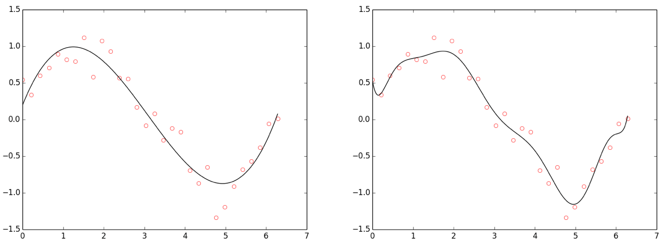
Figure: Overfitting. Points drawn from sin(x) + Gaussian noise. Left: Polynomial fit, degree 3 (cubic; good fit). Right: Polynomial fit, degree 10 (overfit).

Statisticians use the term cross-validation to describe the process of splitting the training data into two (or more) parts, and using one part to fit the model, and the other to assess whether or not it exhibits overfitting. In machine learning, this is more often referred to as a "test-training" approach.

A special form of this approach is longitudinal validation, in which we build the model on data from one time period and then check its performance against data from a later time period, either by partitioning the data available at build time into older and newer data, or by using outcomes collected after the model was built for validation. With longitudinal validation, we seek to verify not only that we did not overfit the characteristics of a particular data sample, but also that the patterns we model are stable over time.

Validating against data for which the outcomes were not known when the model was developed has the additional benefit of eliminating a common class of errors that arises when secondary information about validation outcomes "leaks" during the model building process. Some degree of such leakage—sometimes known as contaminating the validation data—is quite common.

Generalized Overfitting

As its name suggests, overfitting as normally conceived is a failure mode specific to model building, arising when we fit the training data "too well". Here, we are are going to argue that overfitting is an example of a more general failure mode that can be present in any analytical process, especially if we use the process with data other than that used to build it. Our suggested name for this broader class of failures is errors of applicability.

Here are some of the failure modes we are thinking about:

Changes in Distributions of Inputs (and Outputs)

1. New categories. When we develop the analytical process, we see only categories A, B and C in some (categorical) input or output. In operation, we also see category D. At this point our process may fail completely ("crash"), produce meaningless outputs or merely produce less good results.

2. Missing categories. The converse can be a problem too: what if a category disappears? Most prosaically, this might lead to a divide-by-zero error if we've explicitly used each category frequency in a denominator. Subtler errors can also creep in.

3. Extended ranges. For numeric and other ordered data, the equivalent of new categories is values outside the range we saw in the development data. Even if the analysis code runs without incident, the process will be being used in a way that may be quite outside that considered and tested during development, so this can be dangerous.

4. Distributions. More generally, even if the range of the input data doesn't change, its distribution may, either slowly or abruptly. At the very least, this indicates the process is being used in unfamiliar territory.

5. Nulls. Did nulls appear in any fields where there were none when we developed the process? Does the process cater for this appropriately? And are such nulls valid?

6. Higher Dimensional Shifts. Even if the the data ranges and distribution for individual fields don't change, their higher dimensional distributions (correlations) can change significantly. The pair of 2-dimensional distributions below illustrates this point in an extreme way. The distributions of both x and y values on the left and right are identical. But clearly, in 2 dimensions, we see that the space occupied by the two datasets is actually non-overlapping, and on the left x and y are negatively correlated, while on the right they are positively correlated.

   

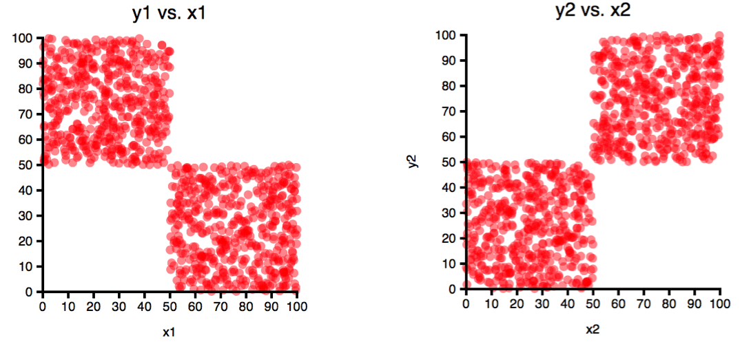
   Figure: The same x and y values are shared between these two plots (i.e. the disibution of x and y is identical in each case). However, the pairing of x and y coordinates is different. A model or other analytical process built with with negatively correlated data like that on the left might not work well for positively correlated data like that on the right. Even if it does work well, you may want to detect and report a fundamental change like this.

7. Time (always marching on). Times and dates are notoriously problematical. There are many issues around date and time formats, many specifically around timezones (and the difference between a local times and times in a fixed time zone, such as GMT or UTC).

   For now, let's assume that we have an input that is a well-defined time, correctly read and analysed in a known timezone—say UTC.¹ Obviously, new data will tend to have later times—sometimes non-overlapping later times. Most often, we need to change these to intervals measured with respect to a moving date (possibly today, or some variable event date, e.g. days since contact). But in other cases, absolute times, or times in a cycle matter. For example, season, time of month or time of day may matter—the last two, probably in local time rather than UTC.

   In handling time, we have to be careful about binnings, about absolute vs. relative measurement (2015-12-11T11:00:00 vs. 299 hours after the start of the current month), universal vs. local time, and appropriate bin boundaries that move or expand with the analytic time window being considered.

   Time is not unique in the way that its range and maximum naturally increase with each new data sample. Most obviously, other counters (such as customer number) and sum-like aggregates may have this same monotonically increasing character, meaning that it should be expected that new, higher (but perhaps not new lower) values will be present in newer data.

Concrete and Abstract Definitions

There's a general issue with choosing values based on data used during development. This concerns the difference between what we will term concrete and abstract values, and what it means to perform "the same" operation on different datasets.

Suppose we decide to handle outliers differently from the rest of the data in a dataset, at least for some part of the analysis. For example, suppose we're looking at flight prices in Sterling and we see the following distribution.

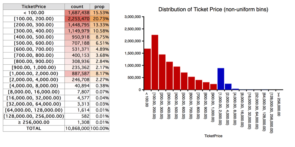
Figure: Ticket prices, in £100 bins to £1,000, then doubling widths to £256,000, with one final bin for prices above £256,000. (On the graph, the £100-width bins are red; the rest are blue.)

On the basis of this, we see that well over 99% of the data has prices under £4,000, and also that while there are a few thousand ticket prices in the £4,000–£32,000 range (most of which are probably real) the final few thousand probably contain bad data, perhaps as a result of currency conversion errors.

We may well want to choose one or more threshold values from the data—say £4,000 in this case—to specify some aspect of our analytical process. We might, for example, use this threshold in the analysis for filtering, outlier reporting, setting a final bin boundary or setting the range for the axes of a graph.

The crucial question here is: How do we specify and represent our threshold value?

• Concrete Value: Our concrete value is £4,000. In the current dataset there are 60,995 ticket prices (0.55%) above this value and 10,807,905 (99.45%) below. (There are no prices of exactly £4,000.) Obviously, if we specify our threshold using this concrete value—£4,000—it will be the same for any dataset we use with the process.

• Abstract Value: Alternatively, we might specify the value indirectly, as a function of the input data. One such abstract specification is the price P below which which 99.45% of ticket prices the dataset lie. If we specify a threshold using this abstract definition, it will vary according to the content of the dataset.

  • In passing, 99.45% is not precise: if we select the bottom 99.45% of this dataset by price we get 10,808,225 records with a maximum price of £4,007.65. The more precise specification is that 99.447046% of the dataset has prices under £4,000.

  • Of course, being human, if we were specifying the value in this way, we would probably round the percentage to 99.5%, and if we did that we would find that we shifted the threshold so that the maximum price below it was £4,186.15, and the minimum price above was £4,186.22.

• Alternative Abstract Specifications: Of course, if we want to specify this threshold abstractly, there are countless other ways we might do it, some fraught with danger.

  Two things we should definitely avoid when working with data like this are means and variances across the whole column, because they will be rendered largely meaningless by outliers. If we blindly calculate the mean, μ, and standard deviation, σ, in this dataset, we get μ=£2,009.85 and σ=£983,956.28. That's because, as we noted previously, there are a few highly questionable ticket prices in the data, including a maximum of £1,390,276,267.42.² Within the main body of the data—the ~99.45% with prices below £4,000.00—the corresponding values are μ=£462.09 and σ=£504.82. This emphasizes how dangerous it would be to base a definition on full-field moments³ such as mean or variance.

  In contrast, the median is much less affected by outliers. In the full dataset, for example the median ticket price is £303.77, while the median of those under £4,000.00 is £301.23. So another reasonably stable abstract definition of a threshold around £4,000.00 would be something like 13 times the median.

The reason for labouring this point around abstract vs. concrete definitions is that it arises very commonly and it is not always obvious which is preferable. Concrete definitions have the advantage of (numeric) consistency between analyses, but may result in analyses that are not well suited to a later dataset, because different choices would have been made if that later data had been considered by the developer of the process. Conversely, abstract definitions often make it easier to ensure that analyses are suitable for a broader range of input datasets, but can make comparability more difficult; they also tend to make it harder to get "nice" human-centric scales, bin boundaries and thresholds (because you end up, as we saw above, with values like £4,186.22, rather than £4,000).

Making a poor choice between abstract and concrete specifications of any data-derived values can lead to large sections of the data being omitted (if filtering is used), or made invisible (if used for axis boundaries), or conversely can lead to non-comparability between results or miscomputations if values are associated with bins having different boundaries in different datasets.

NOTE: A common source of the leakage of information from validation data into training data, as discussed above, is the use of the full dataset to make decisions about thresholds such as those discussed here. To get the full benefit of cross-validation, all modelling decisions need to be made solely on the basis of the training data; even feeding back performance information from the validation data begins to contaminate that data.

Data-derived thresholds and other values can occur almost anywhere in an analytical process, but specific dangers include:

1. Selections (Filters). In designing analytical processes, we may choose to filter values, perhaps to removing outliers or nonsensical values. Over time, the distribution may shift, and these filters may become less appropriate and remove ever-increasing proportions of the data.

   A good example of this we have seen recently involves negative charges. In early versions of ticket price information, almost all charges were positive, and those that were negative were clearly erroneous, so we added a filter to remove all negative charges from the dataset. Later, we started seeing data in which there were many more, and less obviously erroneous negative charges. It turned out that a new data source generated valid negative charges, but we were misled in our initial analysis and the process we built was unsuitable for the new context.

2. Binnings (Bandings, Buckets). Binning data is very common, and it is important to think carefully about when you want bin boundaries to be concrete (common across datasets) and when they should be abstract (computed, and therefore different for different datasets). Quantile binnings (such as deciles), of course, are intrinsically adaptive, though if those are used you have to be aware that any given bin in one dataset may have different boundaries from the "same" bin in another dataset.

3. Statistics. As noted above, some care has to be taken when any statistic is used in the dataset to determine whether it should be recorded algorithmically (as an abstract value) in analysis or numerically (as a concrete value), and particular care should be taken with statistics that are sensitive to outliers.

Other Challenges to Applicability

In addition to the common sources of errors of applicability we have outlined above, we will briefly mention a few more.

1. Non-uniqueness. Is a value that was different for each record in the input data now non-unique?

2. Crazy outliers. Are there (crazy) outliers in fields where there were none before?

3. Actually wrong. Are there detectable data errors in the operational data that were not seen during development?

4. New data formats. Have formats changed, leading to misinterpretation of values?

5. New outcomes. Even more problematical than new input categories or ranges are new outcome categories or a larger range of output values. When we see this, we should almost always re-evaluate our analytical processes.

Four Kinds of Analytical Errors

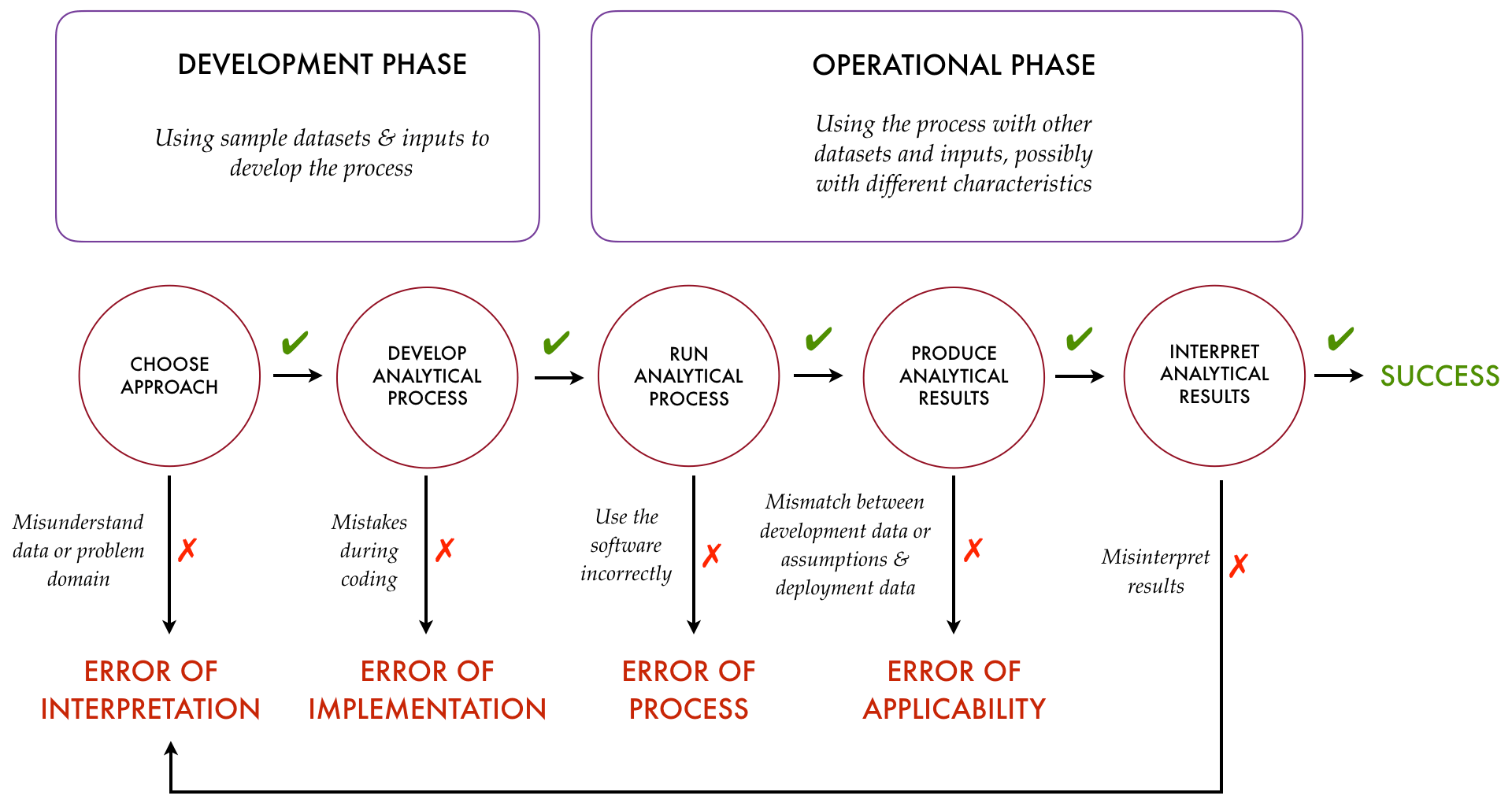
In the overview of TDDA we published in Predictive Analytic Times (available here), we made an attempt to summarize how the four main classes of errors arise with the following diagram:

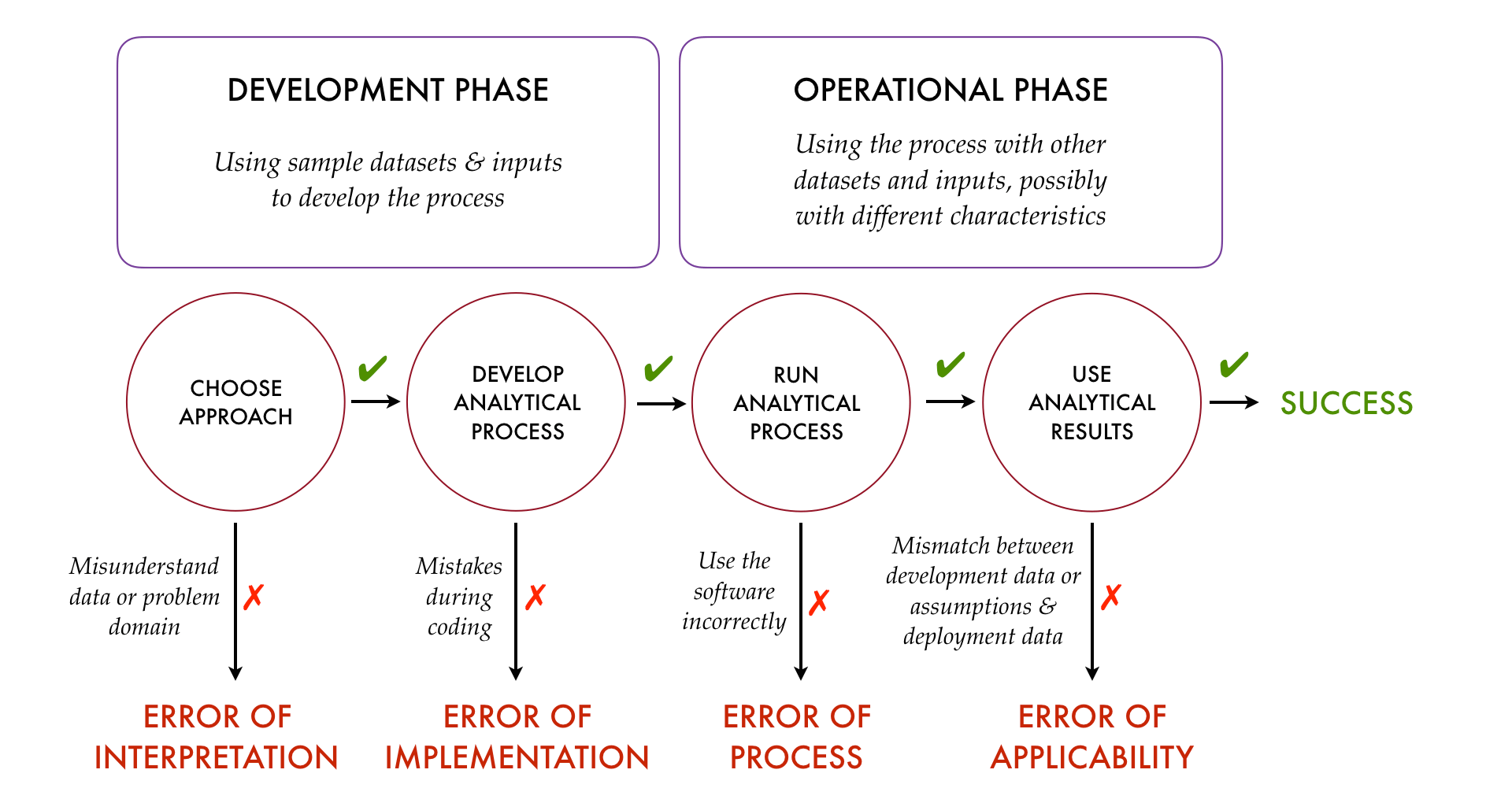
While this was always intended to be a simplification, a particular problem is that it suggests there's no room for errors of interpretation in the operationalization phase, which is far from the case.⁴ Probably a better representation is as follows: