Unix & Linux Survival Guide for Data Science etc.
Posted on Mon 21 February 2022 in TDDA • Tagged with tests, cartoon
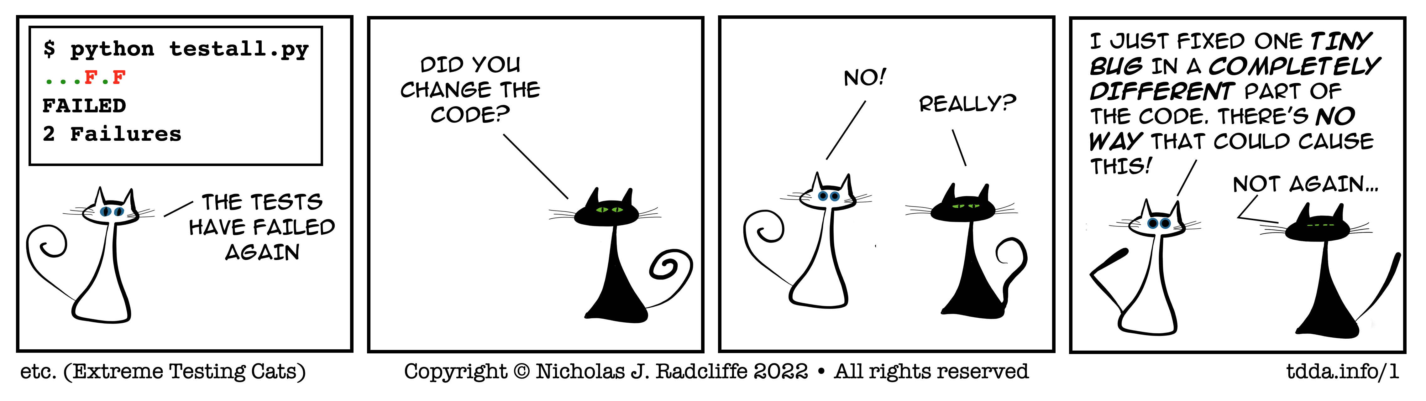
Posted on Mon 21 February 2022 in TDDA • Tagged with tests, cartoon
Posted on Wed 16 February 2022 in TDDA • Tagged with tests, cartoon
Posted on Mon 07 February 2022 in TDDA • Tagged with tests, reference tests, rust
or Why Tests Spontanously Fail
You might think that if you write a program, and don't change anything, then come back a day later (or a decade later) and run it with the same inputs, it would produce the same output. At their core, reference tests exist because this isn't true, and it's useful to find out if code you wrote in the past no longer does the same thing it used to. This post collects together some of reasons the behaviour of code changes over time.1
E1 You updated your compiler/interpreter (Python/R etc.)
E2 You updated libraries used in your code (e.g. from PyPI/CRAN).
E3 You updated the operating system of the machine you're running on.
E4 Someone else updated the operating system or library/compiler etc.
E5 Your code uses some other software on your machine (or another)
machine that has been updated (e.g. a database).
E6 Your code uses an external service whose behaviour has changed
(e.g. calling a web service to get/do something).
E7 You have updated/replaced your hardware.
E8 You run it on different hardware (another machine or OS or OS version
or under a different compiler or...)
E9 You move the code to a different location in the file system.
E10 You have changed something in the file system that messes up the code
e.g.
E11 You run as a different user.
E12 You run from a different directory while leaving the code in the
same place.
E13 You run the code in a different way (e.g. from a script instead
of interactively, or in a scheduler).
E14 A disk fills or some other resource becomes full or depleted.
E15 The load on the machine is higher, and the code runs out of
memory or disk or some other resource; or has a subtle timing
dependency or assumption that fails under load.
E15a The load on the machine is lower, meaning part of your code
runs faster, causing a race condition to behave differently.
[Added 2022-02-17]
E16 The hardware has developed a fault.
E17 A systems manager has changed some limits e.g. disk quotas,
allowed nice levels, a directory service, some permissions or groups...
E18 A shell variable changed, or was created or destroyed.
E19 The locale in which the machine is running changed.
E20 You changed your PYTHONPATH or equivalent.
E21 A new library that you don't use (or didn't think you used)
has appeared in a site-packages or similar location, and was picked
up by your code or something else your code uses.
E22 You updated your editor/IDE and now whenever you load a file it
gets changes in some subtle way that matters (e.g. line endings, blank
lines at the of files, encoding, tabs vs. spaces).
E23 The physical environment has changed in some way that affects
the machine you are running on (e.g. causing it to slow down).
E24 A file has been touched2 and the software determines order
of processing by last update date.
E25 The code uses a password or key that is changed, expires or
is revoked.
E26 The code requires network access and the network is unavailable, slow, or unreliable at the time the test is run.
E27 Almost any of the above (or below), but for a dependency of your code rather than your code itself, e.g. something in a data centre or library.
E28 Your PATH (the list of locations checks for executables) has
changed, or an alias has changed so that the executable you run is
different from before. [Added 2022-02-11]
E29 A different disk or share is mounted, so that even though you
specify the same path, some file that you are using is different from
before. [Added 2022-02-11]
E30 You run the code under a different shell or changed something in a shell startup file. [Added 2022-02-17]
Many of these are illuminated by one of my favourite quote from Beth Andres-Beck:
Mocking in unit tests makes the tests more stable because they don’t break when your code breaks.
— @bethcodes, 2020-12-29T01:26:00Z https://twitter.com/bethcodes/status/1343730015851069440
C1 You think you didn't change the code, but actually you did.
C2 You did change the code, but only in a way that couldn't
possibly change the behaviour in the case you're testing.
C3 You didn't change the code, you fixed a bug.
C4 You didn't change the code, but someone else did.
C5 You didn't change the code, but disk corruption did.
C6 You didn't change the code, but you did update some data it uses.
C7 You pulled the code again from a source-code repository but
C8 You're on the wrong branch.
C9 The system was restored from backup and you lost changes.
C10 You used a hard link to a file and didn't change the file here but
did change it in one of the other linked locations.
C11 You used symbolic links and though your symbolic link
didn't change, the code (or other file or files) it symbolically linked did.
C12 You used a diff tool to compare files, but a difference that
does matter to your code was not detected by the diff tool (e.g. line
endings or capitalization or whitespace).
C13 You are in fact running more tests than previously, or different tests
from the ones you ran previously, without realising it.
C14 You reformatted your code thinking that you were only making
changes to appearance.
C15 You ran a code formatter/beautifier/coding standard enforcement
tool that had a bug in it and changed the meaning.
C16 You believe nothing has changed because git status tells you nothing
has changed, but you are using files that aren't tracked or are ignored.
C17 You think a file hasn't changed because of its timestamp, but the
timestamp is wrong or doesn't mean what you think it means.
C18 A hidden file changed (e.g. a dotfile).
C19 A file that doesn't match a glob pattern you use changed.
C20 The file is in a cloud linked folder (e.g. Dropbox)
and changed remotely. [Added 2025-01-31]
C21 A coding bot changed your code [Added 2025-06-02]
Also from Beth Andres-Beck:
If you have 100% test coverage and your tests use mocks, no you don’t.
— @bethcodes, 2020-12-29T01:51:00Z https://twitter.com/bethcodes/status/1343736477839020032
There is another set of problems that aren't strictly causes of code rusting, but which help to explain a set of related situations every developer has probably experienced, which all fall under the general heading of you aren't running the code you think you are.
M1 The code you're running is not the the version you think it is
(e.g. you're in the wrong directory).
M2 You are running the code on a different server from the one you think
you are (e.g. you haven't realised you're ssh'd in to a different
machine or editing a file over a network).
M3 You're editing the code in one place but running it in another.
M4 You have cross-mounted a file system and it's the wrong file
system or you think you are/aren't using it when you actually
aren't/are (respectively).
M5 Something (e.g. a browser) is caching your code (or some CSS
or an image or something).
M6 The code has in fact run correctly (tests have passed)
but you're look at the wrong output (wrong directory, wrong tab,
wrong URL, wrong window, wrong machine...)
M7 Your compiled code is out-of-sync with your source code, so you're
not running what you think you are.
M8 You're running (or not running) a virtual environment when you
think you are not (or are), respectively.
M9 You're running a virtual environment and not understanding how
it's doing its magic, with the result that you're not using the libraries/code
you think you are.
M10 You use a package manager that's installed the right libraries
into a different Python (or whatever) from the one you think it has.3
M11 You think you haven't changed the code/libraries/Python you're
using, but in fact you did when you updated (what you thought was)
a different virtual (or non-virtual) environment.
M12 You have a conflict between different import directories (e.g.
a local site-packages and a system site-packages), with different
versions of the same library, and aren't importing the one you think you are.
M13 You think the code hasn't changed because you recorded the
version number, but there was a code change that didn't cause the
version number to be changed, or the code has multiple version
numbers, or the code is reporting its version number wrongly, or the
version number actually refers to a number of slightly different
builds that are supposed to have the same behaviour, but don't.
M14 You have defined the same class or method or function or variable
more than once in a language that doesn't mind such things, and are looking
at (and possibly) editing a copy of the relevant function/callable/object
that is masked by the later definition. [Added 2022-09-14]
M15 A web server or application server has your code in memory and
changing or recompiling your code won't have any effect until you restart
that web server or application server. This is really a variation of M5,
but is subtly different because you wouldn't normally think of this as
caching. [Added 2024-03-30]
These are the ones that make you question your sanity.
TIP If what's happening can't be happening, trying introducing a clear syntax error or debug statement or some other change you should be able to see. Then check that it shows up as expected when you're running your code.
Almost every time I think I'm losing my mind when coding, it's because I'm editing and running different code (or viewing results from different code).
T1 Your code has a (usually implicit) date/time dependence in it, e.g.
T2 Time is 'bigger' in some material way that causes a problem, e.g.
T3 While the code is running, daylight savings time starts or stops,
and a measured (local) time interval goes negative.
T4 Your code uses Excel to interpret data and today's a special date
that Excel doesn't (or more likely does) recognize.
T5 The system clock is wrong (perhaps badly wrong); or the system
clock was wrong when you ran it before and is now right.
R1 A resource your code uses (a database, a reference file, a page
on the internet, a web service) returns different data
from the data it always previously returned.
R2 A resource your code uses returns data in a different format
e.g. a different text encoding, different precision, different line endings
(Unix vs. PC vs. Mac), presence or absence of a byte-order marker (BOM) in UTF-8, presence of new characters in Unicode, different normalization of unicode, indented or unindented JSON/XML, different sort order etc.
R3 A resource you depend on returns “the same” data as expected but
something about the interaction is different, e.g. a different status
code or some extra data you can ignore, or some redundant data you
use has been removed.
S1 Your code uses random numbers and doesn't fix the seed.
S2 Your code uses random numbers and does fix the main seed
but not other seeds that get used (e.g. the the seed for numpy is
different from Python's main seed).
S3 A cosmic ray hits the machine and causes a bit flip.
S4 The code is running on a GPU (or even CPU) that does not,
in fact, always produce the same answer (order of execution).
S5 The code is running on a parallel, distributed, or multi-threaded
system and there is inderminacy, a race condition, possible deadlock
or livelock, or any number of other things that might cause indeterminate
behaviour.
S6 Your code assumes something is deterministic or has specified
behaviour that is in fact not determinisic or specified, especially
if that result is the same most but not all of the time, e.g. tie-breaking
in sorts, order of extraction from sets or (unordered) dictionaries,
or the order in which results arrive from asynchronous calls.4
S7 Your code relies on something likely but not certain, e.g. that
two randomly-generated, fairly long IDs will be different from each other.
S8 Your code uses random numbers and does fix the main seed, but
the sequence of random numbers has changed. This has happened with
NumPy, where they realised that one of the sampling functions was
drawing unnecessary samples from the PRNG. In making the sampler more
efficient, they changed the samples that were returned for the same
PRNG seed. [Contributed by Rob Moss
(@rob_models and
@rob_models@mas.to), who "had a quick
search for the relevant issue/changelog item, but it was a long time
ago (~NumPy 1.7, maybe)." He "couldn't find the original NumPy issue,
but here's a similar one: https://github.com/numpy/numpy/issues/14522".
Thanks, Rob!]
[Added 2024-07-19]
I realised there's another whole class of errors of process/errors of interpretation that could lead us to think that code has “rusted” despite not having been changed. These are all broadly the same as one of the explanations offered before, but now for the original run when you thought it worked, rather than for the current or new run, when it fails.
N1 You thought you ran the code before, and that it worked correctly,
but you are mistaken: you didn't run it at all, or it in fact failed
but you did not notice.
N2 You did run the code before, but picked up the output from
a previous state, before you broke it, when it did work.
N3 You did run the code before, and it did produce the
wrong output then as now, but you used a defective procedure
or tool to examine the output then, and failed to realise
it was wrong/failing.
N4 You did run the code before, and it did pass, but you
passed the wrong parameters/inputs/whatever and are now passing
the correct (or different) parameters/inputs/whatever so it now
fails as it would have done then if you had done the same.
If you have think of other reasons code rusts, do let me know and I'll be happy to expand this list (and attribute, of course) ↩
Touching a file (the unix touch command) updates the last
update date on a file without changing its contents. ↩
For this reason, a lot of people prefer to run python -m pip
rather than pip, because this way you can have greater confidence that
the module is getting installed in the site-packages for the version
of python you're actually running. ↩
Most of these kinds of indeterminacy will, in fact, usually be stable given identical inputs on the same machine running the same software, but it can take very little to change that, and should not be relied upon. ↩
This week, a client I'm working for received a large volume of data, and as usual the data was sent as "flat" files—or CSV (comma-separated values1) files, as they are more often called. Everyone hates CSV files, because they are badly specified, contain little metadata and are generally an unreliable way to transfer information accurately. They continue to be used, of course, because they are the lowest-common denominator format and just about everything can read and write them in some fashion.
Some of the problems with CSV files are well captured in a pithy blog post by Jesse Donat entitled Falsehoods Programmers Believe about CSVs.
Among other things, the data we received this week featured:
All of this is a bit frustrating, but far from unusual, and only one of these problems was actually fatal—the use of unquoted, unescaped separators in values, which makes the file inherently ambiguous. I'm almost sure this data was written but not read or validated, because I don't believe the supplier would have been able to read it reliably either.
Metadata
In an ideal world, we'd move away from CSV files, but we also need to recognise not only that this probably won't happen, but that the universality, plain-text nature, grokkability and simplicity of CSV files are all strengths; for all that we might gain using fancier, better-specified formats, we would lose quite a lot too, not least the utility of awk, split, grep and friends in many cases.
So if we can't get away from CSV files, how can we increase reliability when using them? Standardizing might be good, but again, this is going to be hard to achieve. What we might be able to do, however, is to work towards a way of specifying flat files that at least allows a receiver of them to know what to expect, or a generator to know what to write. I've been involved with a few such ideas over the years, and the software my company produces (Miró) used its own non-standard, XML-based way of describing flat files.
What I'm thinking about is trying to produce something more general, less opinionated, and more modern (think JSON, rather than XML, for starters) that addresses more issues. The initial goal would be simply descriptive—to allow a metadata file to be created that accurately describes the specific features of a given flat file so that a reader (human or machine) knows how to interpret it. Over time, this might grow into something bigger. I think obvious things to do after the format is created include:
tdda library
to be able to use this when using CSV files for input
(and perhaps also for output).Together, a smart reader that generates a metadata file for a CSV file (item 4 above) and a validator that validates a CSV file against such a metadata specification (item 5) are very analogous to the current constraint discovery and data verification, respectively, but in the space of CSV files—roughly, "syntactic" conformance—rather than data (or "semantic") correctness.
Miró's Flat File Description format (XMD Files)
Here is an example, from its documentation, of the XMD data files that Miró uses.
<?xml version="1.0" encoding="UTF-8"?>
<dataformat>
    <sep>,</sep>                     <!-- field separator -->
    <null></null>                    <!-- NULL marker -->
    <quoteChar>"</quoteChar>         <!-- Quotation mark -->
    <encoding>UTF-8</encoding>       <!-- any python coding name -->
    <allowApos>True</allowApos>      <!-- allow apostophes in strings -->
    <skipHeader>False</skipHeader>   <!-- ignore the first line of file -->
    <pc>False</pc>                   <!-- Convert 1.2% to 0.012 etc. -->
    <excel>False</excel>             <!-- pad short lines with NULLs -->
    <dateFormat>eurodt</dateFormat>  <!-- Miró date format name -->
    <fields>
        <field extname="mc id" name="ID" type="string"/>
        <field extname="mc nm" name="MachineName" type="int"/>
        <field extname="secs" name="TimeToManufacture" type="real"/>
        <field extname="commission date" name="DateOfCommission"
               type="date"/>
        <field extname="mc cp" name="Completion Time" type="date"
               format="rdt"/>
        <field extname="sh dt" name="ShipDate" type="date" format="rd"/>
        <field extname="qa passed?" name="Passed QA" type="bool"/>
    </fields>
    <requireAllFields>False</requireAllFields>
    <banExtraFields>False</banExtraFields>
</dataformat>
Three things to note immediately about this:
extname is the name in the CSV file (the external name),
while the name is the name
for Miró to use for the field. The semantics of this are slightly
complicated, but allow for renaming of fields on import, and for naming
of fields where there is no external name,
or external names are repeated,
or the external name is otherwise unusable by Miró.
If the CSV file has a header and each field has a different name in the
header, the order of the fields int he XMD file does not matter, but if
there are missing or repeated field names, Miró will use the field
order in the XMD file.Notwithstanding the amazing variety seen in CSV files, as illuminated by Jesse Donat's aforementioned blogpost, most CSV files from mature systems vary only in the ways covered by a few of the items described in the CSV file. The most important things to know about a flat file overall are normally:
,), but pipe (|), tab
and semicolon (;) are also frequently used.Escaping.
How are characters "escaped"? This really covers a set of different
issues, and the XMD file is not rich enough to cover all possibilities.
One aspect is, when strings are quoted, how are quotes in the
string handled? The most common answers are either by preceding
them with an escape character, usually backslash (\), e.g.
"This is an escaped \" character in a string"
or by stuttering:
"This is a stuttered "" character in a string"
Escaping is also a way of including the separator in non-quoted values, like these display prices:
Price,DisplayPrice
100.0,£100.00
1000.0,£1\,000.00
1000000,£1\,000\,000.00
Escaping is also a way of specifying some special characters,
e.g. \n for a newline, \t for a tab etc., and as a result
when an actually backslash is required it is self-escaped
(as \\).
Row Truncation after the last non-null value.
Are rows in which the last value is missing truncated?
Like many CSV writers, Excel writes missing values as blanks
so that 1,,3 is read as 1 for the first field, a missing
value for the second field and 3 for the third field.
More quirkily, when Excel writes out CSV files, if there are
n columns and the last m of them on a row are missing,
Excel will write out only the non-missing values, and no further
separators, so that there will be only n – m values on that line
and only n – m – 1 separators.
This behaviour is hard to describe and (as far as I know) unique
to Excel, so in the
XMD file this is simply marked as <excel>True</excel>.7
Field1 to FieldN if no fieldnames
are available in the flat file or any XMD file.)Per-Field Information
It's always useful and sometimes necessary to specify field types, and as discussed above, sometimes field names. Typing is almost always ambigous, and such ambiguity is increased if there are any bad values in the data. Moreover, in some cases (especially dates and timestamps), it is useful to specify the date format. Although good flat-file readers generally make a reasonable job of inferring types, and often date formats too, it is clearly helpful for a metadata specification to include these.
Just as date formats can vary between fields, other things can vary too, most obviously null indicators (missing value information), quoting and escaping. Moreover, if numeric data is formatted (e.g. including currency indicators, thousand separators etc.) these can all usefully be specified.
Required/Allowed Fields
The final pair of settings in the XMD file look slightly different from
the others, partly because they are phrased as directives rather than
descriptions. requireAllFields, when set, is a directive to Miró
to raise a warning or an error if any of the fields in the XMD file are
not present in the CSV file. Similarly, banExtraFields is a directive
to raise such a warning or error if any fields are found in the CSV file
that are not listed in the XMD file. Miró has several ways to specify
whether infringements result in warnings or errors.
These directives can, however, be recast as declarations. The
banExtraFields directive, when true, can equally be thought of as a
declaration the field list is complete. Similarly, the
requireAllFields directive, when true, can be thought of as a
declaration that the field list is not just describing types that and
formats for fields that might be in the CSV files, but rather that all fields
listed are actually in the file.8
In principle, I think it would probably be better if these descriptions were more obviously descriptive or declarative, but I am struggling to find a pair of words/phrases that would capture that elegantly. At this point I am tempted to retain their imperative nature but make them slightly more symmetrical, perhaps with:
"require-all-fields": true,
"allow-extra-fields": false
Alternatively a more declarative syntax might be something like:
"csv-file-might-omit-fields": false,
"csv-file-might-include-extra-fields": false
The reader might wonder why the fields in the metadata file would ever not correspond exactly to those in file. In practice, it is not uncommon when dealing with relatively "good" CSV files to write an XMD file that specifies types and formats only for fields that trip up the flat-file reader. Conversely, it can be useful to have XMD files that describe a variety of possible files that share field names and types; in those cases, the extra ones do no harm.
What Might a Metadata File Look Like?
The XMD file gets quite a lot of things right:
There are also a few major shortcomings:
Some of these shortcomings reflect the fact that the XMD format was conceived less as a general-purpose flat-file descriptor than a specification as to how Miró should read or write a given flat file, and also a way for Miró to specify how it has written a flat file.
Essentially, I think a good flat-file description format would preserve the good aspects and remedy the faults identified, as well as providing a mechanism for specifying some more esoteric possibilies not mentioned so far.
I'll propose something concrete in subsequent posts.
UPDATE The example metadata was updated on 2025-06-23, to be slightly more interesting and realistic. This coincides with the the post, tdda.serial: Metadata for Flat Files (CSV Files)
Sometimes the separator in a flat file is a character other than a
comma, and you occasionally see .tsv used an extension when the separator
is a tab character, or .psv when the separator is a pipe character (|).
Often, however, a csv extension is still used, and as result the acronym
CSV is sometimes restyled as character-separated values. I had always
heard this extension attributed to Microsoft, but have been unable
to verify this. ↩
To be fair, the notion of different kinds of missing values is reasonable—missing because it wasn't recorded, missing because it was unreadable, missing because it's an undefined result (e.g. mean of no values) etc. But this wasn't that: it was just multiple ways of denoting generic missing values. ↩
by which, of course, I mean as well as ... ↩
There's an interesting question as to whether the CSV format specification should be incorporated as an optional part of a TDDA file, and if so, whether it should simply be a nested section or whether the field-specific components should be merged with TDDA's field sections. There are pros and cons. ↩
Yes, some systems do this. ↩
I know, madness! But such practices occur! ↩
Maybe it should have been called quirks mode ↩
Miró's slightly extended version of TDDA files includes lists of required and allowed fields, which serve a similar purpose to these settings. ↩
Posted on Sun 30 August 2020 in TDDA • Tagged with tests, reference tests, data
I've been dabbling in Swift—Apple's new-ish programming language—recently. One of the things I often do when learning a new language is either to take an existing project in a language I know (usually, Python) and translate it to the new one, or (better) to try a new project, first writing it in Python then translating it. This allows me to separate out debugging the algorithm from debugging my understanding of the new language, and also give me something to test against.
I have a partially finished Python project for analysing chords that I've been starting to translate, and this has led me to begin to experiment with some new extensions to the TDDA library (not yet pushed/published).
It's a bit fragmented and embryonic, but this what I'm thinking about.
Sharing test data between languages
Many tests boil down to "check that passing these inputs to this function1 produces this result". There would be some benefits in sharing the inputs and expected outputs between implementations:
** Looping over test cases **
Standard unit-testing dogma tends to focus on the idea of testing small units using many tests, each containing a single assertion, usually as the last statement in the test.2 The benefit of using a single assertion is that when there's a failure it's very clear what it was, and an earlier failure doesn't prevent a later check (assertion) from being carried out: you get all your failures in one go. Less importantly, it also means that the number of tests executed is the same as the number of assertions tested, which might be useful and psychologically satisfying.
On the other hand, it is extremely common to want to test multiple input-output pairs and it is natural and convenient to collect those together and loop over them. I do this all the time, and the reference testing capability in the TDDA library already helps mitigate some downsides of this approach in some situations.
A common way I do this is to loop over a dictionary or a list of tuples
specifying input-output pairs. For example, if I were testing a function
that did string slicing from the left in python (string[:n])
I might use something like
cases = {
    ('Catherine', 4): 'Cath',
    ('Catherine', -6): 'Cath',  # deliberately wrong, for illustration
    ('', 7): '',
    ('Miró forever', 4): 'Miró',
    ('Miró forever', 0): ' '    # also deliberately wrong
}
for (text, n), expected in cases.items():
    self.assertEqual(left_string(text, n), expected)
In Python this is fine, because tuples, being hashable, can be used
as dictionary keys, and there's something quite intuitive and satisfying
about the cases being presented as lines of the form
input: expected output. But I also often just use nested tuples or lists,
partly as a hangover from older versions of Python in which dictionaries
weren't sorted.3 Here's a full example using tuples:
from tdda.referencetest import ReferenceTestCase

def left_string(s, n):
    return s[:n]


class TestLeft(ReferenceTestCase):
    def testLeft(self):
        cases = (
            (('Catherine', 4), 'Cath'),
            (('Catherine', -6), 'Cath'),    # deliberately wrong, for illustration
            (('', 7), ''),
            (('Miró forever', 4), 'Miró'),
            (('Miró forever', 0), ' ')      # also deliberately wrong
        )
        for (text, n), expected in cases:
            self.assertEqual(left_string(text, n), expected)


if __name__ == '__main__':
    ReferenceTestCase.main()
As noted above, two problems with this are:
'Cath') are repeated.We can see both of these problems if we run this:
$ python3 looptest.py
F
======================================================================
FAIL: testLeft (__main__.TestLeft)
----------------------------------------------------------------------
Traceback (most recent call last):
  File "looptest.py", line 18, in testLeft
    self.assertEqual(left_string(text, n), expected)
AssertionError: 'Cat' != 'Cath'
- Cat
+ Cath
?    +


----------------------------------------------------------------------
Ran 1 test in 0.000s

FAILED (failures=1)
It's actually the second case that failed, and the fifth case would also fail if it ran (since it should produce an empty string, not a space).
A technique I've long used to address the first problem is to include the test case in the equality assertion, replacing
self.assertEqual(actual, expected)
with
self.assertEqual((case, actual), (case, expected))
like so:
def testLeft(self):
    cases = (
        (('Catherine', 4), 'Cath'),
        (('Catherine', -6), 'Cath'),
        (('', 7), ''),
        (('Miró forever', 4), 'Miró'),
        (('Miró forever', 0), ' ')
        )
    for case, expected in cases:
        (text, n) = case
        self.assertEqual((case, left_string(text, n)),
                         (case, expected))
Now when a case fails, we see what the failure is more easily:
$ python3 looptest2.py
F
======================================================================
FAIL: testLeft (__main__.TestLeft)
----------------------------------------------------------------------
Traceback (most recent call last):
  File "looptest2.py", line 20, in testLeft
    (case, expected))
AssertionError: Tuples differ: (('Catherine', -6), 'Cat') != (('Catherine', -6), 'Cath')

First differing element 1:
'Cat'
'Cath'

- (('Catherine', -6), 'Cat')
+ (('Catherine', -6), 'Cath')
?                         +


----------------------------------------------------------------------
Ran 1 test in 0.001s

FAILED (failures=1)
I wouldn't call it beautiful, but it does the job, at least when the inputs and outputs are of a manageable size.
This still leaves the problem that the failure of an earlier case prevents
later cases from running. The TDDA library already addresses this
in the case of file checks, by providing the
assertFilesCorrect (plural) assertion in addition to the
assertFileCorrect (singular); we'll come back to it later.
Returning to the main theme of this post, when there are multiple implementations of software, potentially in different languages, there is some attraction to being able to share the test data—ideally, both the inputs being tested and the expected results.
The project I'm translating is a chord analysis tool focused on
jazz guitar chords, especially moveable ones with no root.
It has various classes, functions and structures concerned with musical
notes, scales, abstract chords, tunings, chord shapes, chord names and
so forth. It includes an easy-to-type text format that
uses # as the sharp sign and b as the flat sign, though on output,
these are usually translated to ♯ and ♭. Below are two simple tests
from the Python code.
For those interested, the first tests a function transpose that
transposes a note by an number of semitones. There's an optional key
parameter which, when provided, is used to decide whether to express
the result as a sharp or flat note (when appropriate).
def testTranspose(self):
    self.assertEqual(transpose('C', 0), 'C')

    self.assertEqual(transpose('C', 1), 'C#')
    self.assertEqual(transpose('C', 1, key='F'), 'Db')
    self.assertEqual(transpose('C#', -1), 'C')
    self.assertEqual(transpose('Db', -1), 'C')

    self.assertEqual(transpose('C', 2), 'D')
    self.assertEqual(transpose('D', -2), 'C')

    self.assertEqual(transpose('C', 3, key='A'), 'D#')
    self.assertEqual(transpose('C', 3), 'Eb')
    self.assertEqual(transpose('C', 3, key='Bb'), 'Eb')

    self.assertEqual(transpose('D#', -3), 'C')
    self.assertEqual(transpose('Eb', -3), 'C')

    self.assertEqual(transpose('C', -1), 'B')
    self.assertEqual(transpose('B', 1), 'C')

    self.assertEqual(transpose('C', -2), 'Bb')
    self.assertEqual(transpose('C', -2, 'E'), 'A#')
    self.assertEqual(transpose('Bb', 2), 'C')
    self.assertEqual(transpose('A#', 2), 'C')

    self.assertEqual(transpose('C', -3), 'A')
    self.assertEqual(transpose('A', 3), 'C')

    self.assertEqual(transpose('G', 4), 'B')
    self.assertEqual(transpose('B', -4), 'G')

    self.assertEqual(transpose('F#', 4), 'Bb')
    self.assertEqual(transpose('F#', 4, 'E'), 'A#')
    self.assertEqual(transpose('Bb', -4), 'F#')
    self.assertEqual(transpose('A#', -4), 'F#')
    self.assertEqual(transpose('Bb', -4, 'F'), 'Gb')
    self.assertEqual(transpose('A#', -4, 'Eb'), 'Gb')

    self.assertEqual(transpose('G', 4), 'B')
    self.assertEqual(transpose('F#', 4), 'Bb')
    self.assertEqual(transpose('F#', 4, 'E'), 'A#')
    self.assertEqual(transpose('B', -4), 'G')
    self.assertEqual(transpose('Bb', -4), 'F#')
    self.assertEqual(transpose('A#', -4), 'F#')
    self.assertEqual(transpose('Bb', -4, 'F'), 'Gb')
    self.assertEqual(transpose('A#', -4, 'F'), 'Gb')
Clearly, this test does not use looping, but does combine some 36 test cases in a single test (dogma be damned!)
A second test is for a function to_flat_equiv, which (again, for
those interested) accepts chord names (in various forms) and—where
the chord's key is sharp, as written—converts them to the equivalent
flat form. (Here, o is one of the ways to indicate a diminished
chord (e.g. Dº) and M is on of the ways of describing a major chord
(also maj or Δ). The function also accepts None as an input
(returned unmodified) and R as an abstract chord with no key
specified (also unmodified).4
def test_to_flat_equiv(self):
    cases = (a
        ('C', 'C'),
        ('C#m', 'Dbm'),
        ('Db7', 'Db7'),
        ('C#M7', 'DbM7'),
        ('Do', 'Do'),
        ('D#M', 'EbM'),
        ('E9', 'E9'),
        ('FmM7', 'FmM7'),
        ('F#mM7', 'GbmM7'),
        ('G', 'G'),
        ('G#11', 'Ab11'),
        ('Ab11', 'Ab11'),
        ('Am11', 'Am11'),
        ('A#+', 'Bb+'),
        ('Bb+', 'Bb+'),
        ('A♯+', 'B♭+'),
        ('B♭+', 'B♭+'),

        (None, None),
        ('R', 'R'),
        ('R#', 'R#'),
        ('Rm', 'Rm'),
        )
    for k, v in cases:
        self.assertEqual(to_flat_equiv(k), v)

    for letter in 'BEPQaz@':
        self.assertRaises(NoteError, to_flat_equiv, letter + '#')
This function uses two loops within the test, one for the good cases and another for eight illegal input cases that raise exceptions. The looping has a clear benefit, but there's no reason to have combined the good and bad test cases in a single test function other than laziness.
In 2020, if we're going to share the test data between implementations,
it hard to look beyond JSON. Here's an extract from a file
scale-tests.json that encapsulates the inputs and expected outputs
for all the tests above:
{
    "transpose": [
        [["C", 0], "C"],

        [["C", 1], "C#"],
        [["C", 1, "F"], "Db"],
        [["C#", -1], "C"],
        [["Db", -1], "C"],

        [["C", 2], "D"],
        [["D", -2], "C"],

        [["C", 3, "A"], "D#"],
        [["C", 3], "Eb"],
        [["C", 3, "Bb"], "Eb"],

        [["D#", -3], "C"],
        [["Eb", -3], "C"],

        [["C", -1], "B"],
        [["B", 1], "C"],

        [["C", -2], "Bb"],
        [["C", -2, "E"], "A#"],
        [["Bb", 2], "C"],
        [["A#", 2], "C"],

        [["C", -3], "A"],
        [["A", 3], "C"],

        [["G", 4], "B"],
        [["B", -4], "G"],

        [["F#", 4], "Bb"],
        [["F#", 4, "E"], "A#"],
        [["Bb", -4], "F#"],
        [["A#", -4], "F#"],
        [["Bb", -4, "F"], "Gb"],
        [["A#", -4, "Eb"], "Gb"],

        [["G", 4], "B"],
        [["F#", 4], "Bb"],
        [["F#", 4, "E"], "A#"],
        [["B", -4], "G"],
        [["Bb", -4], "F#"],
        [["A#", -4], "F#"],
        [["Bb", -4, "F"], "Gb"],
        [["A#", -4, "F"], "Gb"],
    ],
    "flat_equivs": [
        ["C", "C"],
        ["C#m", "Dbm"],
        ["Db7", "Db7"],
        ["C#M7", "DbM7"],
        ["Do", "Do"],
        ["D#M", "EbM"],
        ["E9", "E9"],
        ["FmM7", "FmM7"],
        ["F#mM7", "GbmM7"],
        ["G", "G"],
        ["G#11", "Ab11"],
        ["Ab11", "Ab11"],
        ["Am11", "Am11"],
        ["A#+", "Bb+"],
        ["Bb+", "Bb+"],
        ["A♯+", "B♭+"],
        ["B♭+", "B♭+"],

        [null, null],

        ["R", "R"],
        ["R#", "R#"],
        ["Rm", "Rm"]
    ],
    "flat_equiv_bads": "BEPQaz@"
}
I have a function that reads this uses json.load to read this and
other test data, storing the results in an object with a .scale attribute,
like so:
>>> from moveablechords.utils import ReadJSONTestData
>>> from pprint import pprint
>>> TestData = ReadJSONTestData()
>>> pprint(TestData.scale['transpose'])
[[['C', 0], 'C'],
 [['C', 1], 'C#'],
 [['C', 1, 'F'], 'Db'],
 [['C#', -1], 'C'],
 [['Db', -1], 'C'],
 [['C', 2], 'D'],
 [['D', -2], 'C'],
 [['C', 3, 'A'], 'D#'],
 [['C', 3], 'Eb'],
 [['C', 3, 'Bb'], 'Eb'],
 [['D#', -3], 'C'],
 [['Eb', -3], 'C'],
 [['C', -1], 'B'],
 [['B', 1], 'C'],
 [['C', -2], 'Bb'],
 [['C', -2, 'E'], 'A#'],
 [['Bb', 2], 'C'],
 [['A#', 2], 'C'],
 [['C', -3], 'A'],
 [['A', 3], 'C'],
 [['G', 4], 'B'],
 [['B', -4], 'G'],
 [['F#', 4], 'Bb'],
 [['F#', 4, 'E'], 'A#'],
 [['Bb', -4], 'F#'],
 [['A#', -4], 'F#'],
 [['Bb', -4, 'F'], 'Gb'],
 [['A#', -4, 'Eb'], 'Gb'],
 [['G', 4], 'B'],
 [['F#', 4], 'Bb'],
 [['F#', 4, 'E'], 'A#'],
 [['B', -4], 'G'],
 [['Bb', -4], 'F#'],
 [['A#', -4], 'F#'],
 [['Bb', -4, 'F'], 'Gb'],
 [['A#', -4, 'F'], 'Gb']]
I have also made it so you can get entries using attribute lookup on
the objects, i.e. TestData.scale.transpose rather than
TestData.scale['transpose'], just because it looks more elegant
and readable to me.
A straightforward refactoring of the testTranspose function to use the
JSON-loaded data in TestData.scale would be
def testTranspose2(self):
    for (case, expected) in TestData.scale.transpose:
        if len(case) == 2:
            (note, offset) = case
            self.assertEqual((case, transpose(note, offset)),
                             (case, expected))
        else:
            (note, offset, key) = case
            self.assertEqual((case, transpose(note, offset, key=key)),
                             (case, expected))
In case this isn't self-explanatory
case is ["C", 0] and expected is 'C';note and offset variables; if the
list is of length three the key variable is also set;self.assertEqual(transpose(note, offset), expected),
we're including the case (the tuple of input parameters) on both sides
of the assertion so that if there's a failure, we can see which
case is failing.We can simplify this further since the transpose function has only
one optional (keyword) argument, key, which can also be provided as a third
positional argument. Assuming we don't specifically need to test the
handling of key as a keyword argument, we can combine the two branches
as follows:
def testTranspose3(self):
    for (case, expected) in TestData.scale.transpose:
        self.assertEqual((case, transpose(*case)),
                         (case, expected))
Here, we're using the * operator to unpack5 case into an argument
list for the transpose function.
It probably hasn't escaped your attention that this third version of
testTranspose is rather generic: the same structure would work
for any function f and list of input-output pairs Pairs:
def testAnyOldFunction_f(self):
    for (case, expected) in Pairs:
        self.assertEqual((case, f(*case)), (case, expected))
This makes it fairly easy to add TDDA support. I added prototype support for this that allows us to use an even shorter version of the test:
def testTranspose4(self):
    self.checkFunctionByArgs(transpose, TestData.scale.transpose)
This new checkFunctionByArgs takes a function to test and a list of
input output pairs and runs a slightly fancier version of
testAnyOldFunction. I'll go into extensions in another post, but the
most important difference is that it will report all failures rather
than stopping at the first one.
We can illustrate this by changing the last first and last cases
in TestData.scale['transpose'] to be incorrect, say:
   [[['C', 0], 'Z'],
     ...
    [["A#", -4, "F"], "Zb"]
If we run testTranspose3 using this modified test data,
we get only the first failing case,
and although the test case is listed in the output,
the output isn't particularly easy to
grok.
$ python3 testscale.py
.....F.......
======================================================================
FAIL: testTranspose2 (__main__.TestScale)
----------------------------------------------------------------------
Traceback (most recent call last):
  File "testscale.py", line 22, in testTranspose2
    (case, expected))
AssertionError: Tuples differ: (['C', 0], 'C') != (['C', 0], 'Z')

First differing element 1:
'C'
'Z'

- (['C', 0], 'C')
?             ^

+ (['C', 0], 'Z')
?             ^


----------------------------------------------------------------------
Ran 13 tests in 0.002s

FAILED (failures=1)
But if we use the TDDA's prototype checkFunctionByArgs functionality,
we see both failures and it shows them in a more digestible format:
$ python3 testscale.py
.....

Case transpose('C', 0): failure.
    Actual: 'C'
  Expected: 'Z'


Case transpose('A#', -4, 'F'): failure.
    Actual: 'Gb'
  Expected: 'Zb'
F.......
======================================================================
FAIL: testTranspose4 (__main__.TestScale)
----------------------------------------------------------------------
Traceback (most recent call last):
  File "testscale.py", line 15, in testTranspose4
    self.checkFunctionByArgs(transpose, TestData.scale.transpose)
  File "/Users/njr/python/tdda/tdda/referencetest/referencetest.py", line 899, in checkFunctionByArgs
    self._check_failures(failures, msgs)
  File "/Users/njr/python/tdda/tdda/referencetest/referencetest.py", line 919, in _check_failures
    self.assert_fn(failures == 0, msgs.message())
AssertionError: False is not true :

Case transpose('C', 0): failure.
    Actual: 'C'
  Expected: 'Z'


Case transpose('A#', -4, 'F'): failure.
    Actual: 'Gb'
  Expected: 'Zb'

----------------------------------------------------------------------
Ran 13 tests in 0.001s

FAILED (failures=1)
The failures currently get shown twice, once during execution of the tests and again at the end in the summary, and the test just counts this as a single failure, though these are both things that could be changed.
There are variant forms of the prototype checking function above to handle keyword arguments only and mixed positional and keyword argmuents. There's also a version specifically for single-argument functions, where it's natural not to write the arguments as a tuple, but a simple value.
I think the potential benefits of sharing data between different implementations of the same project are pretty clear. I haven't actually modified the Swift implementation to use the JSON, but I'm sure doing so will be easy and a clear win. I hope the example above also illustrates that good support from testing frameworks can significantly mitigate the downsides of looping over test cases within a single test function. But there are other potential downsides.
The most obvious problem, to me, is that the separation of the test
data from the test it makes it harder to see what's being tested (and
perhaps means you have to trust the framework more, though that is
quite easy to check). Arguably, this is even more true when the test
is reduced to the one-line form in testTranpose4, rather than longer
form in testTranspose2, where the function arguments are unpacked
and named, so that you can see a bit more of what is actually being
passed into the function.
There's a broader point about the utility of tests as a form of documentation. A web search for externalizing test data uncovered this post from Arvind Patil in 2005 in which he proposes something like scheme here for Java (with XML taking the place of JSON, in 2005, of course). Three replies to the post are quite hostile, including the first for Irakli Nadareishvili, who says:
sorry, but this is a quite dangerous anti-pattern. Unit-tests are not simply for testing a piece of code. They carry several, additional, very important roles. One of them is - documentation.
In a well-tested code, unit-tests are the first examples of API usage (API that they test). A TDD-experienced developer can learn a lot about the API, looking at its unit-tests. For the readability and clarity of what unit-test tests, it is very important that test data is in the code and the reader does not have to consistently hop from a configuration file to the test code.
Also, usually boundary conditions for a code (which is what test data commonly is) almost never change, so there is more harm in this "pattern" than gain, indeed.
This is definitely a reasonable concern. Even if code has good documentation,
it is all too common for it to become out of date, whereas (passing) tests,
almost by definition, tend to stay up-to-date with API changes.
We could mitigate this issue quite a lot by hooking into verbose mode
(-v or --verbose) and having it show each call as well as the test
function being run, which seems like a good idea anyway. At the moment, if
you run the scale tests with -v on my chord project like this you get
output like this:
$ python3 testscale.py -v
testAsSmallestIntervals (__main__.TestScale) ... ok
testDeMinorMajors (__main__.TestScale) ... ok
testFretForNoteOnString (__main__.TestScale) ... ok
testNotePairIntervals (__main__.TestScale) ... ok
testRelMajor (__main__.TestScale) ... ok
testTranspose (__main__.TestScale) ... ok
test_are_not_same (__main__.TestScale) ... ok
test_are_same (__main__.TestScale) ... ok
test_are_same_invalids (__main__.TestScale) ... ok
test_flat_equiv (__main__.TestScale) ... ok
test_flat_equiv_bads (__main__.TestScale) ... ok
test_preferred_equiv (__main__.TestScale) ... ok
test_preferred_equiv_bads (__main__.TestScale) ... ok

----------------------------------------------------------------------
Ran 13 tests in 0.002s

OK
but we could (probably) extend this to something more like:6
$ python3 testscale.py -v
testAsSmallestIntervals (__main__.TestScale) ... ok
testDeMinorMajors (__main__.TestScale) ... ok
testFretForNoteOnString (__main__.TestScale) ... ok
testNotePairIntervals (__main__.TestScale) ... ok
testRelMajor (__main__.TestScale) ... ok
testTranspose (__main__.TestScale) ...
    transpose('C', 0): OK
    transpose('C', 1): OK
    transpose('C', 1, 'F'): OK
    transpose('C#', -1): OK
    transpose('Db', -1): OK
    transpose('C', 2): OK
    transpose('D', -2): OK
    transpose('C', 3, 'A'): OK
    transpose('C', 3): OK
    transpose('C', 3, 'Bb'): OK
    transpose('D#', -3): OK
    transpose('Eb', -3): OK
    transpose('C', -1): OK
    transpose('B', 1): OK
    transpose('C', -2): OK
    transpose('C', -2, 'E'): OK
    transpose('Bb', 2): OK
    transpose('A#', 2): OK
    transpose('C', -3): OK
    transpose('A', 3): OK
    transpose('G', 4): OK
    transpose('B', -4): OK
    transpose('F#', 4): OK
    transpose('F#', 4, 'E'): OK
    transpose('Bb', -4): OK
    transpose('A#', -4): OK
    transpose('Bb', -4, 'F'): OK
    transpose('A#', -4, 'Eb'): OK
    transpose('G', 4): OK
    transpose('F#', 4): OK
    transpose('F#', 4, 'E'): OK
    transpose('B', -4): OK
    transpose('Bb', -4): OK
    transpose('A#', -4): OK
    transpose('Bb', -4, 'F'): OK
    transpose('A#', -4, 'F'): OK
... testTranspose (__main__.TestScale): 36 tests: ... ok
test_are_not_same (__main__.TestScale) ... ok
test_are_same (__main__.TestScale) ... ok
test_are_same_invalids (__main__.TestScale) ... ok
test_flat_equiv (__main__.TestScale) ... ok
test_flat_equiv_bads (__main__.TestScale) ... ok
test_preferred_equiv (__main__.TestScale) ... ok
test_preferred_equiv_bads (__main__.TestScale) ... ok

----------------------------------------------------------------------
Ran 49 test cases across 13 tests in 0.002s

OK
I also found this post from Jeremy Wadhams in 2015 on the subject of Sharing unit tests between several language implementations of one spec. It discusses JsonLogic:
JsonLogic is a data format (built on top of JSON) for storing and sharing rules between front-end and back-end code. It's essential that the same rule returns the same result whether executed by the JavaScript client or the PHP client.
Currently the JavaScript client has tests in QUnit, and the PHP client has tests in PHPunit. The vast majority of tests are "given these inputs (rule and data), assert the output equals the expected result."
Jeremy also suggests something very like the scheme above, again using JSON.
I think this has been quite a promising experiment.
It reduced the length of testscale.py from 223 lines to 75, which wasn't
an aim (and carries the potential issues noted above), but which does
make the scope and structure of the tests easier to understand.
It also achieved the primary goal of allowing test data to be shared
between implementations, which seems like a valuable prize.
Eventually, the project might gain a command line in both implementations,
and and that will potentially enable my favourite mode of testing—pairs
of input command lines and expected output. But this is a useful start.
Meanwhile, I will probably refine (and document and test!) the prototype implementations a bit more and then release it.
If you have thoughts, do get in touch.
or, more generally, this callable. ↩
other than, perhaps, and manual teardown in a try...finally
block. ↩
From Python 3.8 on, all Python dictionaries are ordered. This is also the case in CPython implementations from 3.6 onwards. ↩
The function does not accept B# or E#, even though
musically these can be used as alternatives to C and F respectively.
That is outside the scope of this function. ↩
this operation is sometimes called splatting, and sometimes unsplatting or desplatting. ↩
Would I seem like a very old fuddy-duddy if I ask "who writes 'ok' in lower case anyway?" ↩