An Error of Process

Posted on Wed 08 March 2017 in TDDA • Tagged with tdda, errors of process, errors of interpretation

Yesterday, email subscribers to the blog, and some RSS/casual viewers, will have seen a half-finished (in fact, abandoned) post that began to try to characterize success and failure on the crowd-funding platform Kickstarter.

The post was abandoned because I didn't believe its first conclusion, but unfortunately was published by mistake yesterday.

This post explains what happened and tries to salvage a "teachable moment" out of this minor fiasco.

The problem the post was trying to address

Kickstarter is a crowd-funding platform that allows people to back creative projects, usually in exchange for rewards of various kinds. Projects set a funding goal and backers only pay out if the aggregate pledges made match or exceed the funding goal during a funding period—usually 30 days.

Project Phoenix on Kickstarter, from The Icon Factory, seeks to fund the development of a new version of Twitterrific for Mac. Twitterrific was the first independent Twitter client, and was responsible for many of the things that define Twitter today.1 (You were, and are, cordially invited to break off from reading this post to go and back the project before reading on.)

Ollie is the bird in Twitterrific's icon.

At the time I started the post, the project had pledges of $63,554 towards a funding goal of $75,000 (84%) after 13 days, with 17 days to go. This is what the amount raised over time looked like (using data from Kicktraq):
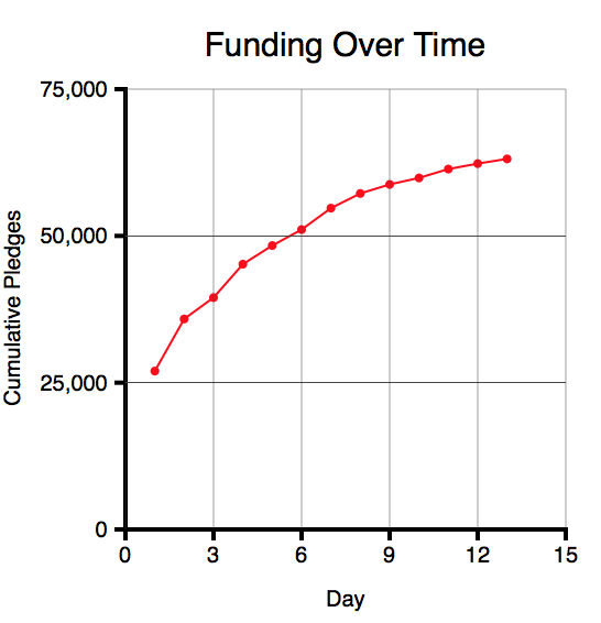
Given that the amount raised was falling each day, and looked asymptotic, questions I was interested in were:

  • How likely was the project to succeed (i.e. to reach its funding goal by day 30? (In fact, it is now fully funded.)
  • How much was the project likely to raise?
  • How likely was the project to reach its stretch goal of $100,000?

The idea was to use some open data from Kickstarter and simple assumptions to try to find out what successful and unsuccessful projects look like.

Data and Assumptions

[This paragraph is unedited from the post yesterday, save that I have made the third item below bold.]

Kickstarter does not have a public API, but is scrapable. The site Web Robots makes available a series of roughly monthly scrapes of Kickstarter data from October 2015 to present; as well as seven older datasets. We have based our analysis on this data, making the following assumptions:

  1. The data is correct and covers all Kickstarter Projects
  2. That we are interpreting the fields in the data correctly
  3. Most critically: if any projects are missing from this data, the missing projects are random. Our analysis is completely invalid if failing projects are removed from the datasets.

[That last point, heavily signalled as critical, turned out not to be the case. As soon as I saw the 99.9% figure below, I went to try to validate that projects didn't go missing from month to month in the scraped data. In fact, they do, all the time, and when I realised this, I abandoned the post. There would have been other ways to try to make the prediction, but they would have been less reliable and required much more work.]

We started with the latest dataset, from 15th February 2017. This included data about 175,085 projects, which break down as follows.

Only projects with a 30-day funding period were included in the comparison, and only those for which we knew the final outcome.

count           is 30 day?
state           no     yes    TOTAL
failed      41,382  42,134   83,516
successful  44,071  31,142   75,213
canceled     6,319   5,463   11,782
suspended      463     363      826
live         2,084   1,664    3,748
TOTAL       94,319  80,766  175,085
-----------------------------------
less live:           1,664
-----------------------------------
Universe            79,102

The table showed that 80,766 of the projects are 30-day, and of these, 79,102 are not live. So this is our starting universe for analysis. NOTE: We deliberately did not exclude suspended or canceled projects, since doing so would have biased our results.

Various fields are available in the JSON data provided by Web Robots. The subset we have used are listed below, together with our interpretation of the meaning of each field:

  • launched_at — Unix timestamp (seconds since 1 January 1970) for the start of the funding period
  • deadline — Unix timestamp for the end of the funding period
  • state — (see above)
  • goal — the amount required to be raised for the project to be funded
  • pledged — the total amount of pledges (today); pledges can only be made during the funding period
  • currency — the currency in which the goal and pledges are made.
  • backers_count — the number of people who have pledged money.

Overall Statistics for 30-day, non-live projects

These are the overall statistics for our 30-day, non-live projects:

succeeded    count        %
no          47,839   60.48%
yes         31,263   39.52%
TOTAL       79,102  100.00%

Just under 40% of them succeed.

But what proportion reach 84% and still fail to reach 100%? According to the detailed data, the answer was just 0.10%, suggesting 99.90% of 30-day projects that reached 84% of their funding goal, at any stage of the campaign went on to be fully funded.

That looked wildly implausible to me, and immediately made me question whether the data I was trying to use was capable of supporting this analysis. In particular, my immediate worry was that projects that looked like they were not going to reach their goal might end up being removed—for whatever reason—more often that those that were on track. Although I have not proved that this is the case, it is clear that projects do quite often disappear between successive scrapes.

To check this, I went back over all the earlier datasets I had collected and extracted the projects that were live in those datasets. There were 47,777 such projects. I then joined those onto the latest dataset to see how many of them were in the latest dataset. 15,276 (31.97%) of the once-live projects were not in the latest data (based on joining on id).

It was at this point I abandoned the blog post.

Error of Process

So what did we learn?

The whole motivation for test-driven data analysis is the observation that data analysis is hard to get right, and most of us make mistakes all the time. We have previously classified these mistakes as

  • errors of interpretation (where we or a consumer of our analysis misunderstand the data, the methods, or our results)
  • errors of implementation (bugs)
  • errors of process (where we make a mistake in using our analytical process, and this leads to a false result being generated or propagated)
  • errors of applicability (where we use an analytical process with data that does not satisfy the requirements or assumptions (explicit or implicit) of the analysis).

We are trying to develop methodologies and tools to reduce the likelihood and impact of each of these kinds of errors.

While we wouldn't normally regard this blog as an analytical process, it's perhaps close enough that we can view this particular error through the TDDA lens. I was writing up the analysis as I did it, fully expecting to generate a useful post. Although I got as far as writing into the entry the (very dubious) 99.9% of 30-day projects that reach 84% funding at any stage on Kickstarter go on to be fully funded, that result immediately smelled wrong and I went off to try to see whether my assumptions about the data were correct. So I was trying hard to avoid an error of interpretation.

But an error of process occurred. This blog is published using Pelican, a static site generator that I mostly quite like. The way Pelican works is posts are (usually) written in Markdown with some metadata at the top. One of the bits of metadata is a Status field, which can either be set to Draft or Published.

When writing the posts, before publishing, you can either run a local webserver to view the output, or actually post them to the main site (on Github Pages, in this case). As long as their status is set to Draft, the posts don't show up as part of the blog in either site (local or on Github), but have to be accessed through a special draft URL. Unfortunately, the draft URL is a little hard to guess, so I generally work with posts with status set to Published until I push them to Github to allow other people to review them before setting them live.

What went wrong here is that the abandoned post had its status left as Published, which was fine until I started the next post (due tomorrow) and pushed that (as draft) to Github. Needless to say, a side-effect of pushing the site with a draft of tomorrow's post was that the abandoned post got pushed too, with its status as Public. Oops!

So the learning for me is that I either have to be more careful with Status (which is optimistic) or I need to add some protection in the publishing process to stop this happening. Realistically, that probably means creating a new Status—Internal—which will get the make process to transmogrify into Published when compiling locally, and Draft when pushing to Github. That should avoid repeats of this particular error of process.


  1. good things, like birds and @names and retweeting; not the abuse. 


Errors of Interpretation: Bad Graphs with Dual Scales

Posted on Mon 20 February 2017 in TDDA • Tagged with tdda, errors of interpretation, graphs

It is a primary responsibility of analysts to present findings and data clearly, in ways to minimize the likelihood of misinterpretation. Graphs should help this, but all too often, if drawn badly (whether deliberately or through oversight) they can make misinterpretation highly likely. I want to illustrate this danger with a unifortunate graph I came across recently in a very interesting—and good, and insightful—article on the US Election.

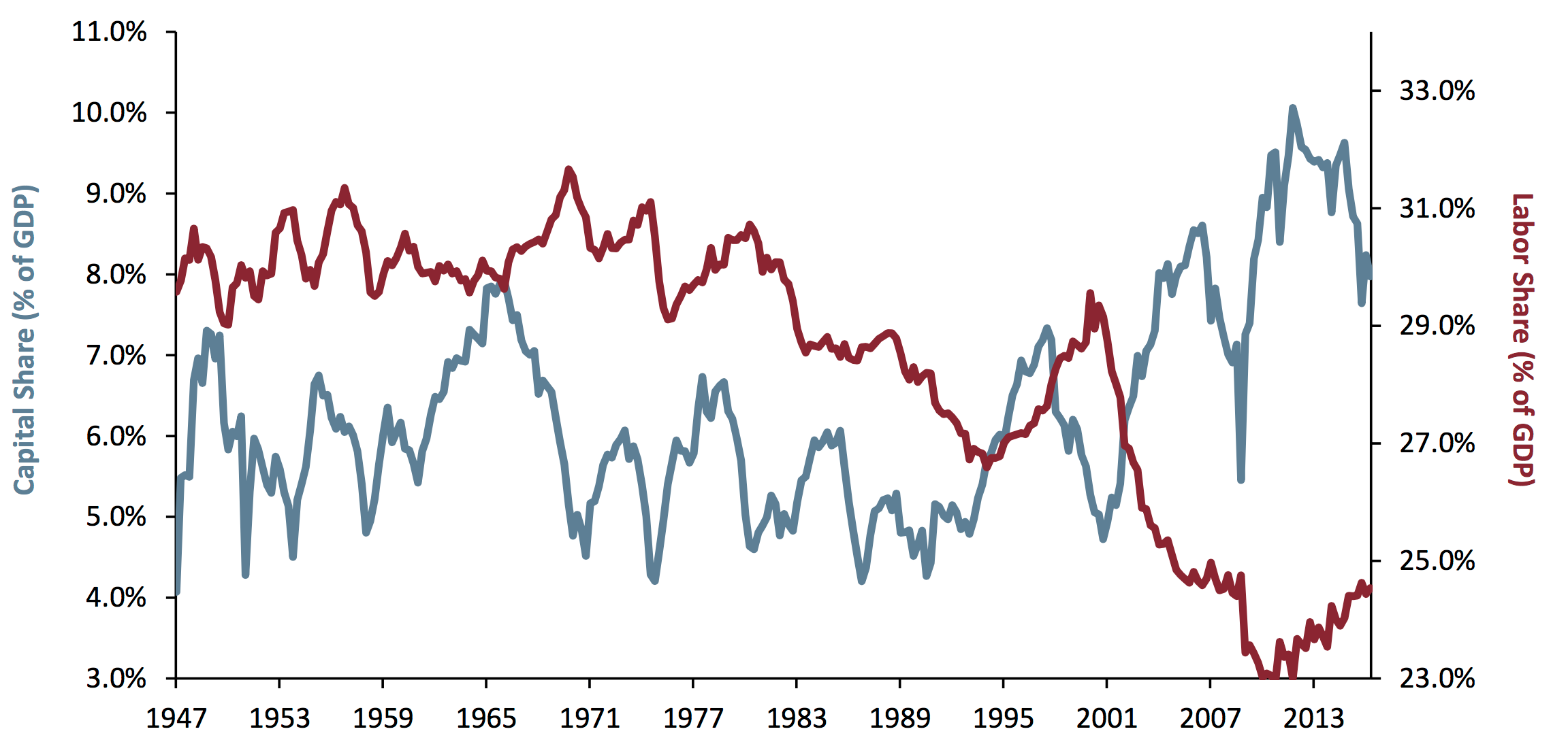
Take a look at this graph, taken from an article called The Road to Trumpsville: The Long, Long Mistreatment of the American Working Class, by Jeremy Grantham.1

Exhibit 1: Corportate Profits and Employee Compensation

In the article, this graph ("Exhibit 1") is described as follows by Grantham:

The combined result is shown in Exhibit 1: the share of GDP going to labor hit historical lows as recently as 2014 and the share going to corporate profits hit a simultaneous high.

Is that what you interpret from the graph? I agree with these words, but they don't really sum up my first reading of the graph. Rather, I think the natural reading of the graph is as follows:

Wow: Labor's share and Capital's share of GDP crossed over, apparently for good, around 2002. Before then, Capital's share was mostly materially lower than Labor's (though they were nearly equal, briefly, in 1965, and crossed for a for a few years in 1995), but over the 66-year period shown Capital's share increased while Labor's fell, until now is taking about four times as much as Labor.

I think something like that is what most people will read from the graph, unless they read it particularly carefully.

But that is not what this graph is saying. In fact, this is one of the most misleading graphs I have ever come across.

If you look carefully, the two lines use different scales: the red one, for Labor, uses the scale on the right, which runs from 23% to about 34%, whereas the blue line for Capital, uses the scale on the left, which runs from 3% to 11%.

Dual-scale graphs are always difficult to read; so difficult, in fact, that my personal recommendation is

Never plot data on two different scales on the same graph.

Not everyone agrees with this, but most people accept that dual-scale graphs are confusing and hard to read. Even, however, by the standards of dual scale graphs, this is bad.

Here are the problems, in roughly decreasing order of importance:

  1. The two lines are showing commensurate2 figures of roughly the same order of magnitude, so could and should have been on the same scale: this isn't a case of showing price against volume, where the units are different, or even a case in which one size in millimetres and another in miles: these are both percentages, of the same thing, all between 4% and 32%.
  2. The graphs cross over when the data doesn't. The very strong suggestion from the graphs that we go from Labor's share of GDP exceeding that of Capital to being radically lower than that of Capital is entirely false.
  3. Despite measuring the same quantity, the magnification is different on the two axes (i.e. the distance on the page between ticks is different, and the percentage-point gap represented by ticks on the two scales is different). As a consequence slopes (gradients) are not comparable.
  4. Neither scale goes to zero.
  5. The position of the two series relative to their scales is inconsistent: the Labor graph goes right down to the x-axis at its minimum (23%) while the Capital graph—whose minimum is also very close to an integer percentage—does not. This adds further to the impression that Labor's share has been absolutely annihilated.
  6. There are no gridlines to help you read the data. (Sure, gridlines are chart junk3, but are especially important when different scales are used, so you have some hope of reading the values.)

I want to be clear: I am not accusing Jeremy Grantham of deliberately plotting the data in a misleading way. I do not believe he intended to distort or manipulate. I suspect he's plotted it this way because stock graphs, which may well be the graphs he most often looks at,4 are frequently plotted with false zeros. Despite this, he has unfortunately plotted the graphs in a way5 that visually distorts the data in almost exactly the way I would choose to do if I wanted to make the points he is making appear even stronger than they are.

I don't have the source numbers, so I have gone through a rather painful exercise, of reading the numbers off the graph (at slightly coarser granularity) so that I can replot the graph as it should, in my opinion, have been plotted in the first place. (I apologise if I have misread any values; transcribing numbers from graphs is tedious and error-prone.) This is the result:

Exhibit 1 (revised): Same Data, with single, zero-based scale (redrawn approximation)

Even after I'd looked carefully at the scales and appreciated all the distortions in the original graph, I was quite shocked to see the data presented neutrally. To be clear: Grantham's textual summary of the data is accurate: a few years ago, Capital's share of GDP (from his figures) were at an all time—albeit not dramatically higher than in 1949 or about 1966—and Labor's share of GDP, a few years ago, was at an all-time low around 23%, down from 30%. But the true picture just doesn't look like the graph Gratham showed. (Again: I feel a bit bad about going on about this graph from such a good article; but the graph encapsulates a number of problematical practices that it makes a perfect illustration.)

How to Lie with Statistics

In 1954, Darrell Huff published a book called How to Lie with Statistics6. Chapter 5 is called The Gee Wizz Graph. His first example is the following graph (neutrally presented) graph:

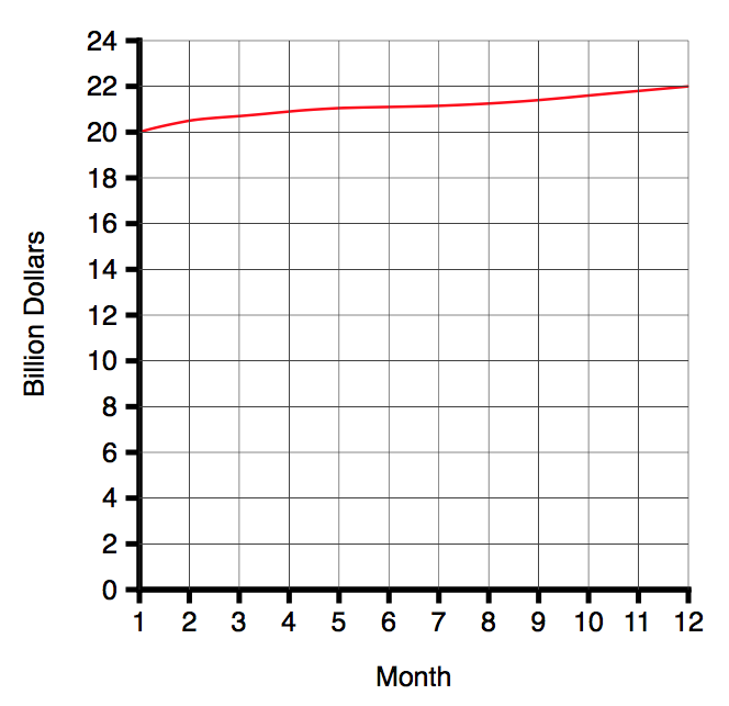
Exhibit 2 (neutral): Sales Data, zero-based scale (redrawn from original)

As Huff says:

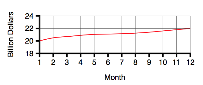
That is very well if all you want to do is convey information. But suppose you wish to win an argument, shock a reader, move him into action, sell him something. For that, this chart lacks schmaltz. Chop off the bottom.

Exhibit 2 (non-zero-based): Sales Data, non-zero-based scale (redrawn from original)

Huff continues:

Thats more like it. (You've saved paper7 too, something to point out if any carping fellow objects to your misleading graphics.)

But there's more, folks:

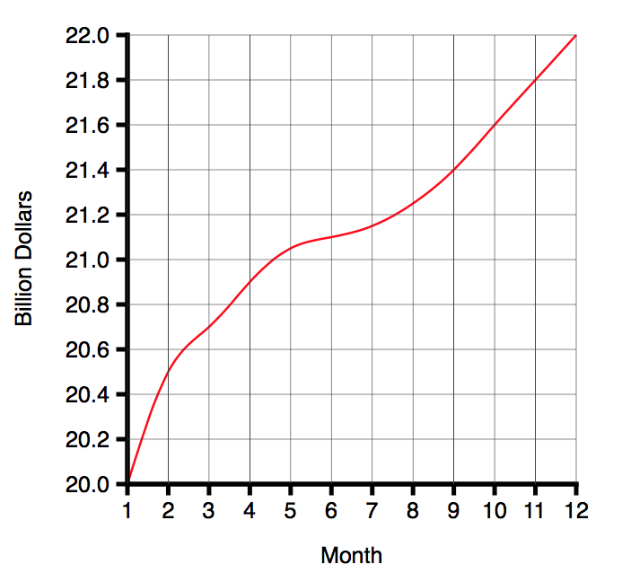
Now that you have practised to deceive, why stop with truncating? You have one more trick available that's worth a dozen of that. It will make your modest rise of ten per cent look livelier than one hundred percent is entitled to look. Simply change the proportion between the ordinate and the abscissa:

Exhibit 2 (non-zero-based, expanded): Sales Data, non-zero-based scale, expanded effect (redrawn from original)

Both of these unfortunate practices are present in Exhibit 1, and that's before we even get to dual scales.

Errors of Interpretation

In our various overviews of test-driven data analysis, (e.g., this summary) we have described four major classes of errors:

  • errors of interpretation
  • errors of implementation (bugs)
  • errors of process
  • errors of applicability

Errors of interpretation can occur at any point in the process: not only are we, the analysts, susceptible to misinterpreting our inputs, our methods, our intermediate results and our outputs, but the recipients of our insights and analyses are in even greater danger of misinterpreting our results, because they have not worked through the process and seen all that we did. As analysts, we have a special responsibility to make our results as clear as possible, and hard to misinterpret. We should assume not that the reader will be diligent, unhurried and careful, reading every number and observing every subtlety, but that she or he will be hurried and will rely on us to have brought out the salient points and to have helped the reader towards the right conclusions.

The purpose of a graph is to bring allow a reader to assimilate large quantities of data, and to understand patterns therein, more quickly and more easily than is possible from tables of numbers. There are strong conventions about how to do that, based on known human strengths and weaknesses as well as commonsense "fair treatment" of different series.

However well intentioned, Exhibit 1 fails in every respect: I would guess very few casual readers would get an accurate impression from the data as presented.

If data scientists had the equivalent of a Hippocratic Oath, it would be something like:

First, do not mislead.


  1. The Road to Trumpsville: The Long, Long Mistreatment of the American Working Class, by Jeremy Grantham, in the GMO Quarterly Newsletter, 4Q, 2016. https://www.gmo.com/docs/default-source/public-commentary/gmo-quarterly-letter.pdf 

  2. two variables are commensurate if they are measured in the same units and it is meaningful to make a direct comparison between them. 

  3. Tufte describes all ink on a graph that is not actually plotting data "chart junk", and advocates "maximizing data ink" (the amount of the ink on a graph actually devoted to plotting the data points) and minimizing chart junk. These are excellent principles. The Visual Display of Quantitative Information, Edward R. Tufte, Graphics Press (Cheshire, Connecticut) 1983. 

  4. Mr Grantham works for GMO, a "global investment management firm". https://gmo.com 

  5. chosen to use a plot, if he isn't responsible for the plot 

  6. How to Lie with Statistics, Darrell Huff, published Victor Gollancz, 1954. Republished, 1973, by Pelican Books. 

  7. Obviously the "saving paper" argument had more force in 1954, and the constant references to "him", "he" and "fellows" similarly stood out less than they do today. 


TDDA 1-pager

Posted on Fri 10 February 2017 in TDDA • Tagged with tdda

We have written a 1-page summary of some of the core ideas in TDDA.

It is available as a PDF from stochasticsolutions.com/pdf/TDDA-One-Pager.pdf.


Coverage information for Rexpy

Posted on Tue 31 January 2017 in TDDA • Tagged with tdda, regular expressions

Rexpy Stats

We previously added rexpy to the Python tdda module. Rexpy is used to find regular expressions from example strings.

One of the most common requests from Rexpy users has been for information regarding how many examples each resulting regular expression matches.

We have now added a few methods to Rexpy to support this.

Currently this is only available in the Python library for Rexpy, available as part of the tdda module, with either

pip install tdda

or

git clone https://github.com/tdda/tdda.git

Needless to say, we also plan to use this functionality in the online version of Rexpy in the future.

Rexpy: Quick Recap

The following example shows simple use of Rexpy from Python:

$ python
>>> from tdda import rexpy
>>>
>>> corpus = ['123-AA-971', '12-DQ-802', '198-AA-045', '1-BA-834']
>>> for r in rexpy.extract(corpus):
>>>    print(r)
>>>
^\d{1,3}\-[A-Z]{2}\-\d{3}$

In this case, Rexpy found a single regular expression that matched all the strings, but in many cases it returns a list of regular expressions, each covering some subset of the examples.

The way the algorithm currently works, in most cases1 each example will match only one regular expression, but in general, some examples might match more than one pattern. So we've designed the new functionality to work even when this is the case. We've provided three new methods on the Extractor class, which gives a more powerful API than the simple extract function.

Here's an example based on one of Rexpy's tests:

>>> urls2 = [
    'stochasticsolutions.com/',
    'apple.com/',
    'stochasticsolutions.com/',  # actual duplicate
    'https://www.stochasticsolutions.co.uk/',
    'https://www.google.co.uk/',
    'https://www.google.com',
    'https://www.google.com/',
    'https://www.guardian.co.uk/',
    'https://www.guardian.com',
    'https://www.guardian.com/',
    'https://www.stochasticsolutions.com',
    'web.stochasticsolutions.com',
    'https://www.stochasticsolutions.com',
    'tdda.info',
    'gov.uk',
    'https://web.web',
]
>>> x = rexpy.Extractor(urls2)
>>> for r in x.results.rex:
>>>    print(r)

^[a-z]{3,4}\.[a-z]{2,4}$
^[a-z]+\.com\/$
^[a-z]{3,4}[\.\/\:]{1,3}[a-z]+\.[a-z]{3}$
^[a-z]{4,5}\:\/\/www\.[a-z]+\.com$
^http\:\/\/www\.[a-z]{6,8}\.com\/$
^http\:\/\/www\.[a-z]+\.co\.uk\/$

As you can see, Rexpy has produced six different regular expressions, some of which should probably be collapsed together. The Extractor object we have created has three new methods available.

The New Coverage Methods

The simplest new method is coverage(dedup=False), which returns a list of the number of matches for each regular expression returned, in the same order as the regular expressions in x.results.rex. So:

>>> print(x.coverage())
[2, 3, 2, 4, 2, 3]

is the list of frequencies for the six regular expressions given, in order. So the pairings are illustrated by:

>>> for k, n in zip(x.results.rex, x.coverage()):
        print('%d examples are matched by %s' % (n, k))

2 examples are matched by ^[a-z]{3,4}\.[a-z]{2,4}$
3 examples are matched by ^[a-z]+\.com\/$
2 examples are matched by ^[a-z]{3,4}[\.\/\:]{1,3}[a-z]+\.[a-z]{3}$
4 examples are matched by ^[a-z]{4,5}\:\/\/www\.[a-z]+\.com$
2 examples are matched by ^http\:\/\/www\.[a-z]{6,8}\.com\/$
3 examples are matched by ^http\:\/\/www\.[a-z]+\.co\.uk\/$

The optional dedup parameter, when set to True, requests deduplicated frequencies, i.e. ignoring any duplicate strings passed in (remembering that Rexpy strips whitespace from both ends of input strings). In this case, there is just one duplicate string (stochasticsolutions.com/). So:

>>> print(x.coverage(dedup=True))
[2, 2, 2, 4, 2, 3]

where the second number (the matches for ^[a-z]+\.com\/$) is now 2, because stochasticsolutions.com/ has been deduplicated.

We can also find the total number of examples, with or without duplicates, by calling the n_examples(dedup=False) method:

>>> print(x.n_examples())
16
>>> print(x.n_examples(dedup=True))
15

But what we will probably normally be most interested in doing is sorting the regular expressions from highest to lowest coverage, ignoring any examples matched by an earlier pattern in cases where they do overlap. That's exactly what the incremental_coverage(dedup=False) method does for us. It returns an ordered dictionary.

>>> for (k, n) in x.incremental_coverage().items():
        print('%d: %s' % (n, k))
4: ^[a-z]{4,5}\:\/\/www\.[a-z]+\.com$
3: ^[a-z]+\.com\/$
3: ^http\:\/\/www\.[a-z]+\.co\.uk\/$
2: ^[a-z]{3,4}[\.\/\:]{1,3}[a-z]+\.[a-z]{3}$
2: ^[a-z]{3,4}\.[a-z]{2,4}$
2: ^http\:\/\/www\.[a-z]{6,8}\.com\/$

This is our sixteen input strings (including duplicates), and the number of examples matched by this expression, not matched by any previous expression. (As noted earlier, that caveat probably won't make any difference at the moment, but it will in future versions.) So, to be explicit, this is saying:

  • The regular expression that matches most examples is: ^[a-z]{4,5}\:\/\/www\.[a-z]+\.com$ which matches 4 of the 16 strings.

  • Of the remaining 12 examples, 3 are matched by ^[a-z]+\.com\/$.

  • Of the remaining 9 examples, 3 more are matched by ^http\:\/\/www\.[a-z]+\.co\.uk\/$

  • and so on.

Note, that in the case of ties, Rexpy sorts regular expressions as strings to break ties.

We can get the deduplicated numbers if we prefer:

>>> for (k, n) in x.incremental_coverage(dedup=True).items():
        print('%d: %s' % (n, k))
4: ^[a-z]{4,5}\:\/\/www\.[a-z]+\.com$
3: ^http\:\/\/www\.[a-z]+\.co\.uk\/$
2: ^[a-z]+\.com\/$
2: ^[a-z]{3,4}[\.\/\:]{1,3}[a-z]+\.[a-z]{3}$
2: ^[a-z]{3,4}\.[a-z]{2,4}$
2: ^http\:\/\/www\.[a-z]{6,8}\.com\/$

That's all the new functionality for now. Let us know how you get on, and if you find any problems. And tweet your email address to @tdda0 if you want to join the TDDA Slack to discuss anything around the subject of test-driven data analysis.

[NOTE: This post was updated on 10.2.2017 after an update to the rexpy library changed function and attribute names from "sequential" (which was not very descriptive) to "incremental", which is better.]


  1. In fact, probably in all cases, currently 


The New ReferenceTest class for TDDA

Posted on Thu 26 January 2017 in TDDA • Tagged with tdda, constraints, rexpy

Since the last post, we have extended the reference test functionality in the Python tdda library. Major changes (as of version 0.2.5, at the time of writing) include:

  • Introduction of a new ReferenceTest class that has significantly more functionality from the previous (now deprecated) WritableTestCase.
  • Support for pytest as well as unittest.
  • Available from PyPI with pip install tdda, as well as from Github.
  • Support for comparing CSV files.
  • Support for comparing pandas DataFrames.
  • Support for preprocessing results before comparison (beyond simply dropping lines) in reference tests.
  • Greater consistency between parameters and options for all comparison methods
  • Support for categorizing kinds of reference data and rewriting only nominated categories (with -w or --write)
  • More (meta) tests of the reference test functionality.

Background: reference tests and WritableTestCase

We previously introduced the idea of a reference test with an example in the post First Test, and then when describing the WritableTestCase library. A reference test is essentially the TDDA equivalent of a software system test (or integration test), and is characterized by:

  • normally testing a relatively large unit of analysis functionality (up to and including whole analytical processes)
  • normally generating one or more large or complex outputs that are complex to verify (e.g. datasets, tables, graphs, files etc.)
  • sometimes featuring unimportant run-to-run differences that mean testing equality of actual and expected output will often fail (e.g. files may contain date stamps, version numbers, or random identifiers)
  • often being impractical to generate by hand
  • often needing to be regenerated automatically (after verification!) when formats change, when bugs are fixed or when understanding changes.

The old WritableTestCase class that we made available in the tdda library provided support for writing, running and updating such reference tests in Python by extending the unittest.TestCase class and providing methods for writing reference tests and commands for running (and, where necessary, updating the reference results used by) reference tests.

Deprecating WritableTestCase in Favour of ReferenceTest

Through our use of reference testing in various contexts and projects at Stochastic Solutions, we have ended up producing three different implementations of reference-test libraries, each with different capabilities. We also become aware that an increasing number of Python developers have a marked preference for pytest over unittest, and wanted to support that more naturally. The new ReferenceTest class brings together all the capabilities we have developed, standardizes them and fills in missing combinations while providing idiomatic patterns for using it both in the context of unittest and pytest.

We have no immediate plans to remove WritableTestCase from the tdda library (and, indeed, continue use it extensively ourselves), but encourage people to adopt ReferenceTest instead as we believe it is superior in all respects.

Availability and Installation

You can now install the tdda module with pip:

pip install tdda

and the source remains available under an MIT licence from github with

git clone https://github.com/tdda/tdda.git

The tdda library works under Python 2.7 and Python 3 and includes reference test functionality mentionedabove, constraint discovery and verification, including a Pandas version and automatic discovery of regular expressions from examples (rexpy, also available online at here).

After installation, you can run TDDA's tests as follows:

$ python -m tdda.testtdda
............................................................................
----------------------------------------------------------------------
Ran 76 tests in 0.279s

Getting example code

However you have obtained the tdda module, you can get a copy of its reference test examples by running the command

$ python -m tdda.referencetest.examples

which will place them in a referencetest-examples subdirectory of your current directory. Alternatively, you can specify that you want them in a particular place with

$ python -m tdda.referencetest.examples /path/to/particular/place

There are variations for getting examples for the constraint generation and validation functionality, and for regular expression extraction (rexpy)

$ python -m tdda.constraints.examples [/path/to/particular/place]
$ python -m tdda.rexpy.examples [/path/to/particular/place]

Example use of ReferenceTest from unittest

Here is a cut-down example of how to use the ReferenceTest class with Python's unittest, based on the example in referencetest-examples/unittest. For those who prefer pytest, there is a similar pytest-ready example in referencetest-examples/pytest.

from __future__ import unicode_literals

import os
import sys
import tempfile

from tdda.referencetest import ReferenceTestCase

# ensure we can import the generators module in the directory above,
# wherever that happens to be
FILE_DIR = os.path.abspath(os.path.dirname(__file__))
PARENT_DIR = os.path.dirname(FILE_DIR)
sys.path.append(PARENT_DIR)

from generators import generate_string, generate_file

class TestExample(ReferenceTestCase):
    def testExampleStringGeneration(self):
        actual = generate_string()
        self.assertStringCorrect(actual, 'string_result.html',
                                 ignore_substrings=['Copyright', 'Version'])

    def testExampleFileGeneration(self):
        outdir = tempfile.gettempdir()
        outpath = os.path.join(outdir, 'file_result.html')
        generate_file(outpath)
        self.assertFileCorrect(outpath, 'file_result.html',
                               ignore_patterns=['Copy(lef|righ)t',
                                                'Version'])

TestExample.set_default_data_location(os.path.join(PARENT_DIR, 'reference'))


if __name__ == '__main__':
    ReferenceTestCase.main()

Notes

  1. These tests illustrate comparing a string generated by some code to a reference string (stored in a file), and testing a file generated by code to a reference file.

  2. We need to tell the ReferenceTest class where to find reference files used for comparison. The call to set_default_data_location, straight after defining the class, does this.

  3. The first test generates the string actual and compares it to the contents of the file string_result.html in the data location specified (../reference). The ignore_substrings parameter specifies strings which, when encountered, cause these lines to be omitted from the comparison.

  4. The second test instead writes a file to a temporary directory (but using the same name as the reference file). In this case, rather than ignore_strings we have used an ignore_patterns parameter to specify regular expressions which, when matched, cause lines to be disregarded in comparisons.

  5. There are a number of other parameters that can be added to the various assert... methods to allow other kinds of discrepancies between actual and generated files to be disregarded.

Running the reference tests: Success, Failure and Rewriting

If you just run the code above, or the file in the examples, you should see output like this:

$ python test_using_referencetestcase.py
..
----------------------------------------------------------------------
Ran 2 tests in 0.003s

OK

or, if you use pytest, like this:

$ pytest
============================= test session starts ==============================
platform darwin -- Python 2.7.11, pytest-3.0.2, py-1.4.31, pluggy-0.3.1
rootdir: /Users/njr/tmp/referencetest-examples/pytest, inifile:
plugins: hypothesis-3.4.2
collected 2 items

test_using_referencepytest.py ..

=========================== 2 passed in 0.01 seconds ===========================

If you then edit generators.py in the directory above and make some change to the HTML in the generate_string and generate_file functions preferably non-semantic changes, like adding an extra space before the > in </html>) and then rerun the tests, you should get failures. Changing just the generate_string function:

$ python unittest/test_using_referencetestcase.py
.1 line is different, starting at line 33
Expected file /Users/njr/tmp/referencetest-examples/reference/string_result.html
Note exclusions:
    Copyright
    Version
Compare with "diff /var/folders/w7/lhtph66x7h33t9pns0616qk00000gn/T/actual-string_result.html
/Users/njr/tmp/referencetest-examples/reference/string_result.html".
F
======================================================================
FAIL: testExampleStringGeneration (__main__.TestExample)
----------------------------------------------------------------------
Traceback (most recent call last):
  File "unittest/test_using_referencetestcase.py", line 62, in testExampleStringGeneration
    ignore_substrings=['Copyright', 'Version'])
  File "/Users/njr/python/tdda/tdda/referencetest/referencetest.py", line 527, in assertStringCorrect
    self.check_failures(failures, msgs)
  File "/Users/njr/python/tdda/tdda/referencetest/referencetest.py", line 709, in check_failures
    self.assert_fn(failures == 0, '\n'.join(msgs))
AssertionError: 1 line is different, starting at line 33
Expected file /Users/njr/tmp/referencetest-examples/reference/string_result.html
Note exclusions:
    Copyright
    Version
Compare with "diff /var/folders/w7/lhtph66x7h33t9pns0616qk00000gn/T/actual-string_result.html
/Users/njr/tmp/referencetest-examples/reference/string_result.html".


    ----------------------------------------------------------------------
    Ran 2 tests in 0.005s

As expected, the string test now fails, and the ReferenceTest library suggests a command you can use to diff the output: because the test failed, it wrote the actual output to a temporary file. (It reports the failure twice, once as it occurs and once at the end. This is deliberate as it's convenient to see it when it happens if the tests take any non-trivial amount of time to run, and convenient to collect together all the failures at the end too.)

Because these are HTML files, I would probably instead open them both (using the open command on Mac OS) and visually inspect them. In these case, the pages look identical, and diff will confirm that the changes are only those we expect:

$ diff /var/folders/w7/lhtph66x7h33t9pns0616qk00000gn/T/actual-string_result.html
/Users/njr/tmp/referencetest-examples/reference/string_result.html
5,6c5,6
<     Copyright (c) Stochastic Solutions, 2016
<     Version 1.0.0

>     Copyright (c) Stochastic Solutions Limited, 2016
>     Version 0.0.0
33c33
< </html >
—
> </html>

In this case

  • We see that the copyright and version lines are different, but we used ignore_strings to avoid say that's OK
  • It shows us the extra space before the close tag.

If we are happy that the new output is OK and should replace the previous reference test, you can rerun with the -W (or --write-all).

$ python unittest/test_using_referencetestcase.py -W
Written /Users/njr/tmp/referencetest-examples/reference/file_result.html
.Written /Users/njr/tmp/referencetest-examples/reference/string_result.html
.
----------------------------------------------------------------------
Ran 2 tests in 0.003s

OK

Now if you run them again without -W, the tests should all pass.

You can do the same with pytest, except that in this case you need to use

pytest --write-all

because pytest does not allow short flags.

Other kinds of tests

Since this post is already quite long, we won't go through all the other options, parameters and kinds of tests in detail, but will mention a few other points:

  • In addition to assertStringCorrect and assertFileCorrect there are various other methods available:

    • assertFilesCorrect for checking that multiple files are as expected
    • assertCSVFileCorrect for checking a single CSV file
    • assertCSVFilesCorrect for checking multiple CSV files
    • assertDataFramesEqual to check equality of Pandas DataFrames
    • assertDataFrameCorrect to check a data frame matches data in a CSV file.
  • Where appropriate, assert methods accept the various optional parameters, including:

    • lstrip — ignore whitespace at start of files/strings (default False)
    • rstrip — ignore whitespace at end of files/strings (default False)
    • kind — optional category for test; these can be used to allow selective rewriting of test output with the -w/--write flag
    • preprocess — function to call on expected and actual data before comparing results

We'll add more detail in future posts.

If you'd like to join the slack group where we discuss TDDA and related topics, DM your email address to @tdda on Twitter and we'll send you an invitation.